Scikit-Learn 教程:如何安装与 Scikit-Learn 示例
什么是 Scikit-learn?
Scikit-learn 是一个用于机器学习的开源 Python 库。它支持最先进的算法,如 KNN、XGBoost、随机森林和 SVM。它构建在 NumPy 之上。Scikit-learn 被广泛用于 Kaggle 竞赛以及知名科技公司。它有助于数据预处理、降维(参数选择)、分类、回归、聚类和模型选择。
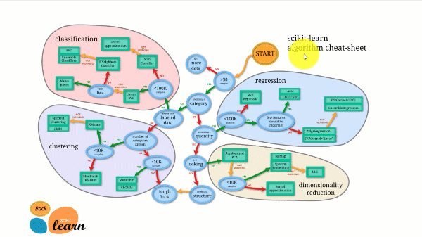
Scikit-learn 拥有所有开源库中最棒的文档。它在 https://scikit-learn.cn/stable/tutorial/machine_learning_map/index.html 提供交互式图表。
Scikit-learn 并不难用,并且能提供出色的结果。然而,scikit learn 不支持并行计算。虽然可以用它来运行深度学习算法,但这并非最优解决方案,尤其是当您知道如何使用 TensorFlow 时。
如何下载和安装 Scikit-learn
现在,在本 Python Scikit-learn 教程中,我们将学习如何下载和安装 Scikit-learn。
选项 1: AWS
scikit-learn 可在 AWS 上使用。请 参考 预装了 scikit-learn 的 Docker 镜像。
要使用开发版本,请在 Jupyter 中使用以下命令:
import sys
!{sys.executable} -m pip install git+git://github.com/scikit-learn/scikit-learn.git
选项 2: 使用 Anaconda 的 Mac 或 Windows
有关 Anaconda 安装,请参阅 https://guru99.com.cn/download-install-tensorflow.html。
最近,scikit 的开发者发布了一个开发版本,解决了当前版本常见的用户问题。我们发现使用开发版本比当前版本更方便。
如何使用 Conda 环境安装 scikit-learn
如果您使用 conda 环境安装了 scikit-learn,请按照步骤更新到版本 0.20。
步骤 1) 激活 tensorflow 环境
source activate hello-tf
步骤 2) 使用 conda 命令删除 scikit lean
conda remove scikit-learn
步骤 3) 安装开发版本。
安装 scikit learn 开发版本以及必要的库。
conda install -c anaconda git
pip install Cython
pip install h5py
pip install git+git://github.com/scikit-learn/scikit-learn.git
注意:Windows 用户需要安装 Microsoft Visual C++ 14。您可以从 此处 获取。
Scikit-Learn 机器学习示例
本 Scikit 教程分为两部分:
- 使用 scikit-learn 进行机器学习
- 使用 LIME 信任您的模型
第一部分详细介绍了如何构建管道、创建模型和调整超参数;第二部分则提供了模型选择方面的最先进技术。
步骤 1) 导入数据
在本 Scikit learn 教程中,您将使用 adult 数据集。
有关此数据集的背景信息,请参考。如果您有兴趣了解更多描述性统计信息,请使用 Dive and Overview 工具。
请参阅 本教程 了解更多关于 Dive and Overview 的信息。
您可以使用 Pandas 导入数据集。请注意,您需要将连续变量的类型转换为 float 格式。
此数据集包含八个分类变量。
分类变量列在 CATE_FEATURES 中。
- workclass
- education
- marital
- occupation
- relationship
- race
- sex
- native_country
此外,还有六个连续变量。
连续变量列在 CONTI_FEATURES 中。
- age
- fnlwgt
- education_num
- capital_gain
- capital_loss
- hours_week
请注意,我们手动填充列表是为了让您更好地了解我们正在使用哪些列。构造分类或连续变量列表的更快方法是使用
## List Categorical
CATE_FEATURES = df_train.iloc[:,:-1].select_dtypes('object').columns
print(CATE_FEATURES)

## List continuous
CONTI_FEATURES =  df_train._get_numeric_data()
print(CONTI_FEATURES)
以下是导入数据的代码:
# Import dataset
import pandas as pd

## Define path data
COLUMNS = ['age','workclass', 'fnlwgt', 'education', 'education_num', 'marital',
           'occupation', 'relationship', 'race', 'sex', 'capital_gain', 'capital_loss',
           'hours_week', 'native_country', 'label']
### Define continuous list
CONTI_FEATURES  = ['age', 'fnlwgt','capital_gain', 'education_num', 'capital_loss', 'hours_week']
### Define categorical list
CATE_FEATURES = ['workclass', 'education', 'marital', 'occupation', 'relationship', 'race', 'sex', 'native_country']

## Prepare the data
features = ['age','workclass', 'fnlwgt', 'education', 'education_num', 'marital',
           'occupation', 'relationship', 'race', 'sex', 'capital_gain', 'capital_loss',
           'hours_week', 'native_country']

PATH = "https://archive.ics.uci.edu/ml/machine-learning-databases/adult/adult.data"

df_train = pd.read_csv(PATH, skipinitialspace=True, names = COLUMNS, index_col=False)
df_train[CONTI_FEATURES] =df_train[CONTI_FEATURES].astype('float64')
df_train.describe()
| age | fnlwgt | education_num | capital_gain | capital_loss | hours_week | |
|---|---|---|---|---|---|---|
| 计数 | 32561.000000 | 3.256100e+04 | 32561.000000 | 32561.000000 | 32561.000000 | 32561.000000 |
| 平均值 | 38.581647 | 1.897784e+05 | 10.080679 | 1077.648844 | 87.303830 | 40.437456 |
| std | 13.640433 | 1.055500e+05 | 2.572720 | 7385.292085 | 402.960219 | 12.347429 |
| min | 17.000000 | 1.228500e+04 | 1.000000 | 0.000000 | 0.000000 | 1.000000 |
| 25% | 28.000000 | 1.178270e+05 | 9.000000 | 0.000000 | 0.000000 | 40.000000 |
| 50% | 37.000000 | 1.783560e+05 | 10.000000 | 0.000000 | 0.000000 | 40.000000 |
| 75% | 48.000000 | 2.370510e+05 | 12.000000 | 0.000000 | 0.000000 | 45.000000 |
| max | 90.000000 | 1.484705e+06 | 16.000000 | 99999.000000 | 4356.000000 | 99.000000 |
您可以检查 native_country 特征的唯一值计数。您可以看到只有一个家庭来自 Holand-Netherlands。这个家庭不会给我们带来任何信息,但会在训练过程中引发错误。
df_train.native_country.value_counts()
United-States                 29170
Mexico                          643
?                               583
Philippines                     198
Germany                         137
Canada                          121
Puerto-Rico                     114
El-Salvador                     106
India                           100
Cuba                             95
England                          90
Jamaica                          81
South                            80
China                            75
Italy                            73
Dominican-Republic               70
Vietnam                          67
Guatemala                        64
Japan                            62
Poland                           60
Columbia                         59
Taiwan                           51
Haiti                            44
Iran                             43
Portugal                         37
Nicaragua                        34
Peru                             31
France                           29
Greece                           29
Ecuador                          28
Ireland                          24
Hong                             20
Cambodia                         19
Trinadad&Tobago                  19
Thailand                         18
Laos                             18
Yugoslavia                       16
Outlying-US(Guam-USVI-etc)       14
Honduras                         13
Hungary                          13
Scotland                         12
Holand-Netherlands                1
Name: native_country, dtype: int64
您可以排除此无信息行。
## Drop Netherland, because only one row
df_train = df_train[df_train.native_country != "Holand-Netherlands"]
接下来,您将连续特征的位置存储在一个列表中。您将在下一步中使用它来构建管道。
下面的代码将遍历 CONTI_FEATURES 中的所有列名,获取其位置(即其编号),然后将其附加到一个名为 conti_features 的列表中。
## Get the column index of the categorical features
conti_features = []
for i in CONTI_FEATURES:
    position = df_train.columns.get_loc(i)
    conti_features.append(position)
print(conti_features)
[0, 2, 10, 4, 11, 12]
下面的代码执行与上面相同的工作,但针对分类变量。下面的代码重复了您之前所做的,只是使用了分类特征。
## Get the column index of the categorical features
categorical_features = []
for i in CATE_FEATURES:
    position = df_train.columns.get_loc(i)
    categorical_features.append(position)
print(categorical_features)
[1, 3, 5, 6, 7, 8, 9, 13]
您可以查看数据集。请注意,每个分类特征都是一个字符串。您不能将字符串值输入模型。您需要使用虚拟变量转换数据集。
df_train.head(5)
事实上,您需要为特征中的每个组创建一个列。首先,您可以运行下面的代码来计算所需的总列数。
print(df_train[CATE_FEATURES].nunique(),
      'There are',sum(df_train[CATE_FEATURES].nunique()), 'groups in the whole dataset')
workclass          9
education         16
marital            7
occupation        15
relationship       6
race               5
sex                2
native_country    41
dtype: int64 There are 101 groups in the whole dataset
如上所示,整个数据集包含 101 个组。例如,workclass 特征有九个组。您可以使用以下代码可视化组名:
unique() 返回分类特征的唯一值。
for i in CATE_FEATURES:
    print(df_train[i].unique())
['State-gov' 'Self-emp-not-inc' 'Private' 'Federal-gov' 'Local-gov' '?'
 'Self-emp-inc' 'Without-pay' 'Never-worked']
['Bachelors' 'HS-grad' '11th' 'Masters' '9th' 'Some-college' 'Assoc-acdm'
 'Assoc-voc' '7th-8th' 'Doctorate' 'Prof-school' '5th-6th' '10th'
 '1st-4th' 'Preschool' '12th']
['Never-married' 'Married-civ-spouse' 'Divorced' 'Married-spouse-absent'
 'Separated' 'Married-AF-spouse' 'Widowed']
['Adm-clerical' 'Exec-managerial' 'Handlers-cleaners' 'Prof-specialty'
 'Other-service' 'Sales' 'Craft-repair' 'Transport-moving'
 'Farming-fishing' 'Machine-op-inspct' 'Tech-support' '?'
 'Protective-serv' 'Armed-Forces' 'Priv-house-serv']
['Not-in-family' 'Husband' 'Wife' 'Own-child' 'Unmarried' 'Other-relative']
['White' 'Black' 'Asian-Pac-Islander' 'Amer-Indian-Eskimo' 'Other']
['Male' 'Female']
['United-States' 'Cuba' 'Jamaica' 'India' '?' 'Mexico' 'South'
 'Puerto-Rico' 'Honduras' 'England' 'Canada' 'Germany' 'Iran'
 'Philippines' 'Italy' 'Poland' 'Columbia' 'Cambodia' 'Thailand' 'Ecuador'
 'Laos' 'Taiwan' 'Haiti' 'Portugal' 'Dominican-Republic' 'El-Salvador'
 'France' 'Guatemala' 'China' 'Japan' 'Yugoslavia' 'Peru'
 'Outlying-US(Guam-USVI-etc)' 'Scotland' 'Trinadad&Tobago' 'Greece'
 'Nicaragua' 'Vietnam' 'Hong' 'Ireland' 'Hungary']
因此,训练数据集将包含 101 + 7 列。最后七列是连续特征。
Scikit-learn 可以处理转换。这分两步完成:
- 首先,您需要将字符串转换为 ID。例如,State-gov 将具有 ID 1,Self-emp-not-inc ID 2,依此类推。LabelEncoder 函数会为您完成此操作。
- 将每个 ID 转换为新列。如前所述,该数据集有 101 个组 ID。因此,将有 101 列用于捕获所有分类特征的组。Scikit-learn 有一个名为 OneHotEncoder 的函数来执行此操作。
步骤 2)创建训练/测试集
现在数据集准备好了,我们可以将其拆分为 80/20。
80% 用于训练集,20% 用于测试集。
您可以使用 train_test_split。第一个参数是特征的 DataFrame,第二个参数是标签的 DataFrame。您可以使用 test_size 指定测试集的大小。
from sklearn.model_selection import train_test_split
X_train, X_test, y_train, y_test = train_test_split(df_train[features],
                                                    df_train.label,
                                                    test_size = 0.2,
                                                    random_state=0)
X_train.head(5)
print(X_train.shape, X_test.shape)
(26048, 14) (6512, 14)
步骤 3)构建管道
管道使输入模型的数据更加一致。
其思想是将原始数据放入“管道”中以执行操作。
例如,对于当前数据集,您需要标准化连续变量并将分类数据进行转换。请注意,您可以在管道内执行任何操作。例如,如果数据集中有“NA”,您可以将其替换为均值或中位数。您还可以创建新变量。
您可以选择:硬编码这两个过程,或创建一个管道。第一种选择可能导致数据泄露并随时间产生不一致。更好的选择是使用管道。
from sklearn.preprocessing import StandardScaler, OneHotEncoder, LabelEncoder
from sklearn.compose import ColumnTransformer, make_column_transformer
from sklearn.pipeline import make_pipeline
from sklearn.linear_model import LogisticRegression
管道将在输入逻辑分类器之前执行两个操作:
- 标准化变量:`StandardScaler()`
- 转换分类特征:OneHotEncoder(sparse=False)
您可以使用 make_column_transformer 执行这两个步骤。此函数在 scikit-learn 的当前版本 (0.19) 中不可用。使用当前版本无法在管道中执行标签编码器和独热编码器。这是我们决定使用开发版本的原因之一。
make_column_transformer 易于使用。您需要定义要应用转换的列以及要执行的转换。例如,要标准化连续特征,您可以这样做:
- conti_features、StandardScaler() 在 make_column_transformer 中。
- conti_features:包含连续变量的列表
- StandardScaler:标准化变量
make_column_transformer 中的 OneHotEncoder 对象会自动编码标签。
preprocess = make_column_transformer(
    (conti_features, StandardScaler()),
    ### Need to be numeric not string to specify columns name
    (categorical_features, OneHotEncoder(sparse=False))
)
您可以使用 fit_transform 测试管道是否正常工作。数据集的形状应为:26048, 107
preprocess.fit_transform(X_train).shape
(26048, 107)
数据转换器已准备就绪。您可以使用 make_pipeline 创建管道。一旦数据被转换,您就可以输入逻辑回归。
model = make_pipeline(
    preprocess,
    LogisticRegression())
使用 scikit-learn 训练模型非常简单。您需要使用 fit 对象,前面加上管道,即 model。您可以使用 scikit-learn 库中的 score 对象打印准确率。
model.fit(X_train, y_train)
print("logistic regression score: %f" % model.score(X_test, y_test))
logistic regression score: 0.850891
最后,您可以使用 predict_proba 预测类别。它返回每个类别的概率。请注意,它们的总和为一。
model.predict_proba(X_test)
array([[0.83576663, 0.16423337],
       [0.94582765, 0.05417235],
       [0.64760587, 0.35239413],
       ...,
       [0.99639252, 0.00360748],
       [0.02072181, 0.97927819],
       [0.56781353, 0.43218647]])
步骤 4)在网格搜索中使用我们的管道
调整超参数(决定网络结构如隐藏单元的变量)可能非常繁琐且耗时。
评估模型的一种方法是更改训练集的大小并评估性能。
您可以重复此方法十次以查看分数指标。然而,这太费力了。
相反,scikit-learn 提供了一个函数来执行参数调整和交叉验证。
交叉验证
交叉验证意味着在训练期间,训练集会被分成 n 个折叠(folds),然后对模型进行 n 次评估。例如,如果 cv 设置为 10,则训练集将训练和评估十次。在每次迭代中,分类器随机选择九个折叠来训练模型,第十个折叠用于评估。
网格搜索
每个分类器都有需要调整的超参数。您可以尝试不同的值,或者设置一个参数网格。如果您访问 scikit-learn 官方网站,可以看到逻辑分类器有不同的参数可以调整。为了加快训练速度,我们选择调整 C 参数。它控制正则化参数。它应该是正数。较小的值会使正则化器获得更高的权重。
您可以使用 GridSearchCV 对象。您需要创建一个包含要调整的超参数的字典。
您列出超参数,然后是您想要尝试的值。例如,要调整 C 参数,您可以使用:
- ‘logisticregression__C’: [0.1, 1.0, 1.0]:参数前面是分类器名称(小写)和两个下划线。
模型将尝试四个不同的值:0.001、0.01、0.1 和 1。
您使用 10 折进行模型训练:cv=10。
from sklearn.model_selection import GridSearchCV
# Construct the parameter grid
param_grid = {
    'logisticregression__C': [0.001, 0.01,0.1, 1.0],
    }
您可以使用参数网格 gri 和 cv 通过 GridSearchCV 训练模型。
# Train the model
grid_clf = GridSearchCV(model,
                        param_grid,
                        cv=10,
                        iid=False)
grid_clf.fit(X_train, y_train)
输出
GridSearchCV(cv=10, error_score='raise-deprecating',
       estimator=Pipeline(memory=None,
     steps=[('columntransformer', ColumnTransformer(n_jobs=1, remainder='drop', transformer_weights=None,
         transformers=[('standardscaler', StandardScaler(copy=True, with_mean=True, with_std=True), [0, 2, 10, 4, 11, 12]), ('onehotencoder', OneHotEncoder(categorical_features=None, categories=None,...ty='l2', random_state=None, solver='liblinear', tol=0.0001,
          verbose=0, warm_start=False))]),
       fit_params=None, iid=False, n_jobs=1,
       param_grid={'logisticregression__C': [0.001, 0.01, 0.1, 1.0]},
       pre_dispatch='2*n_jobs', refit=True, return_train_score='warn',
       scoring=None, verbose=0)
要访问最佳参数,请使用 best_params_。
grid_clf.best_params_
输出
{'logisticregression__C': 1.0}
在用四种不同的正则化值训练模型后,最佳参数为:
print("best logistic regression from grid search: %f" % grid_clf.best_estimator_.score(X_test, y_test))
来自网格搜索的最佳逻辑回归:0.850891
要访问预测概率:
grid_clf.best_estimator_.predict_proba(X_test)
array([[0.83576677, 0.16423323],
       [0.9458291 , 0.0541709 ],
       [0.64760416, 0.35239584],
       ...,
       [0.99639224, 0.00360776],
       [0.02072033, 0.97927967],
       [0.56782222, 0.43217778]])
使用 scikit-learn 的 XGBoost 模型
让我们尝试 Scikit-learn 示例,在市场上最好的分类器之一上进行训练。XGBoost 是随机森林的改进。该分类器的理论背景超出了本 Python Scikit 教程的范围。请记住,XGBoost 赢得了许多 Kaggle 竞赛。对于中等大小的数据集,它的性能可以与深度学习算法相媲美,甚至更好。
该分类器训练起来很困难,因为它需要调整的参数很多。当然,您可以使用 GridSearchCV 来为您选择参数。
相反,让我们看看如何用更好的方法找到最佳参数。GridSearchCV 可能很繁琐,而且如果传递的值很多,训练起来会非常慢。搜索空间随着参数数量的增加而增长。一个更可取的解决方案是使用 RandomizedSearchCV。此方法包括在每次迭代后随机选择每个超参数的值。例如,如果分类器训练 1000 次迭代,则评估 1000 个组合。它的工作原理与 GridSearchCV 大致相同。
您需要导入 xgboost。如果库未安装,请使用 pip3 install xgboost 或
use import sys
!{sys.executable} -m pip install xgboost
在 Jupyter 环境中
下一步,
import xgboost
from sklearn.model_selection import RandomizedSearchCV
from sklearn.model_selection import StratifiedKFold
本 Scikit Python 教程的下一步包括指定要调整的参数。您可以参考官方文档查看所有要调整的参数。为了本 Python Sklearn 教程的方便,我们只选择两个超参数,每个超参数有两个值。XGBoost 需要很长时间来训练,网格中包含的超参数越多,您需要等待的时间就越长。
params = {
        'xgbclassifier__gamma': [0.5, 1],
        'xgbclassifier__max_depth': [3, 4]
        }
我们用 XGBoost 分类器构建了一个新的管道。我们选择定义 600 个估计器。请注意,n_estimators 是一个可以调整的参数。较高的值可能导致过拟合。您可以自行尝试不同的值,但请注意这可能需要数小时。我们使用其他参数的默认值。
model_xgb = make_pipeline(
    preprocess,
    xgboost.XGBClassifier(
                          n_estimators=600,
                          objective='binary:logistic',
                          silent=True,
                          nthread=1)
)
您可以使用 Stratified K-Folds 交叉验证器来改进交叉验证。这里我们只构建了三个折叠以加快计算速度,但降低了质量。在家中将此值增加到 5 或 10 以改进结果。
我们选择在四次迭代中训练模型。
skf = StratifiedKFold(n_splits=3,
                      shuffle = True,
                      random_state = 1001)

random_search = RandomizedSearchCV(model_xgb,
                                   param_distributions=params,
                                   n_iter=4,
                                   scoring='accuracy',
                                   n_jobs=4,
                                   cv=skf.split(X_train, y_train),
                                   verbose=3,
                                   random_state=1001)
随机搜索已准备就绪,您可以训练模型。
#grid_xgb = GridSearchCV(model_xgb, params, cv=10, iid=False)
random_search.fit(X_train, y_train)
Fitting 3 folds for each of 4 candidates, totalling 12 fits
[CV] xgbclassifier__max_depth=3, xgbclassifier__gamma=0.5 ............
[CV] xgbclassifier__max_depth=3, xgbclassifier__gamma=0.5 ............
[CV] xgbclassifier__max_depth=3, xgbclassifier__gamma=0.5 ............
[CV] xgbclassifier__max_depth=4, xgbclassifier__gamma=0.5 ............
[CV]  xgbclassifier__max_depth=3, xgbclassifier__gamma=0.5, score=0.8759645283888057, total= 1.0min
[CV] xgbclassifier__max_depth=4, xgbclassifier__gamma=0.5 ............
[CV]  xgbclassifier__max_depth=3, xgbclassifier__gamma=0.5, score=0.8729701715996775, total= 1.0min
[CV]  xgbclassifier__max_depth=3, xgbclassifier__gamma=0.5, score=0.8706519235199263, total= 1.0min
[CV] xgbclassifier__max_depth=4, xgbclassifier__gamma=0.5 ............
[CV] xgbclassifier__max_depth=3, xgbclassifier__gamma=1 ..............
[CV]  xgbclassifier__max_depth=4, xgbclassifier__gamma=0.5, score=0.8735460094437406, total= 1.3min
[CV] xgbclassifier__max_depth=3, xgbclassifier__gamma=1 ..............
[CV]  xgbclassifier__max_depth=3, xgbclassifier__gamma=1, score=0.8722791661868018, total=  57.7s
[CV] xgbclassifier__max_depth=3, xgbclassifier__gamma=1 ..............
[CV]  xgbclassifier__max_depth=3, xgbclassifier__gamma=1, score=0.8753886905447426, total= 1.0min
[CV] xgbclassifier__max_depth=4, xgbclassifier__gamma=1 ..............
[CV]  xgbclassifier__max_depth=4, xgbclassifier__gamma=0.5, score=0.8697304768486523, total= 1.3min
[CV] xgbclassifier__max_depth=4, xgbclassifier__gamma=1 ..............
[CV]  xgbclassifier__max_depth=4, xgbclassifier__gamma=0.5, score=0.8740066797189912, total= 1.4min
[CV] xgbclassifier__max_depth=4, xgbclassifier__gamma=1 ..............
[CV]  xgbclassifier__max_depth=3, xgbclassifier__gamma=1, score=0.8707671043538355, total= 1.0min
[CV]  xgbclassifier__max_depth=4, xgbclassifier__gamma=1, score=0.8729701715996775, total= 1.2min
[Parallel(n_jobs=4)]: Done  10 out of  12 | elapsed:  3.6min remaining:   43.5s
[CV]  xgbclassifier__max_depth=4, xgbclassifier__gamma=1, score=0.8736611770125533, total= 1.2min
[CV]  xgbclassifier__max_depth=4, xgbclassifier__gamma=1, score=0.8692697535130154, total= 1.2min
[Parallel(n_jobs=4)]: Done  12 out of  12 | elapsed:  3.6min finished
/Users/Thomas/anaconda3/envs/hello-tf/lib/python3.6/site-packages/sklearn/model_selection/_search.py:737: DeprecationWarning: The default of the `iid` parameter will change from True to False in version 0.22 and will be removed in 0.24. This will change numeric results when test-set sizes are unequal. DeprecationWarning)
RandomizedSearchCV(cv=<generator object _BaseKFold.split at 0x1101eb830>,
          error_score='raise-deprecating',
          estimator=Pipeline(memory=None,
     steps=[('columntransformer', ColumnTransformer(n_jobs=1, remainder='drop', transformer_weights=None,
         transformers=[('standardscaler', StandardScaler(copy=True, with_mean=True, with_std=True), [0, 2, 10, 4, 11, 12]), ('onehotencoder', OneHotEncoder(categorical_features=None, categories=None,...
       reg_alpha=0, reg_lambda=1, scale_pos_weight=1, seed=None,
       silent=True, subsample=1))]),
          fit_params=None, iid='warn', n_iter=4, n_jobs=4,
          param_distributions={'xgbclassifier__gamma': [0.5, 1], 'xgbclassifier__max_depth': [3, 4]},
          pre_dispatch='2*n_jobs', random_state=1001, refit=True,
          return_train_score='warn', scoring='accuracy', verbose=3)
正如您所见,XGBoost 的得分比之前的逻辑回归更好。
print("Best parameter", random_search.best_params_)
print("best logistic regression from grid search: %f" % random_search.best_estimator_.score(X_test, y_test))
Best parameter {'xgbclassifier__max_depth': 3, 'xgbclassifier__gamma': 0.5}
best logistic regression from grid search: 0.873157
random_search.best_estimator_.predict(X_test)
array(['<=50K', '<=50K', '<=50K', ..., '<=50K', '>50K', '<=50K'], dtype=object)
在 scikit-learn 中使用 MLPClassifier 创建 DNN
最后,您可以使用 scikit-learn 训练深度学习算法。方法与其他分类器相同。该分类器可在 MLPClassifier 中找到。
from sklearn.neural_network import MLPClassifier
我们定义了以下深度学习算法:
- Adam 优化器
- Relu 激活函数
- Alpha = 0.0001
- 批量大小为 150
- 两个隐藏层,分别有 100 和 50 个神经元。
model_dnn = make_pipeline(
    preprocess,
    MLPClassifier(solver='adam',
                  alpha=0.0001,
                  activation='relu',
                    batch_size=150,
                    hidden_layer_sizes=(200, 100),
                    random_state=1))
您可以更改层数以改进模型。
model_dnn.fit(X_train, y_train)
  print("DNN regression score: %f" % model_dnn.score(X_test, y_test))
DNN 回归得分:0.821253
LIME:信任您的模型
现在您有了一个好的模型,您需要一个工具来信任它。机器学习算法,尤其是随机森林和神经网络,众所周知是黑盒算法。换句话说,它能工作,但没人知道为什么。
三位研究人员提出了一种很棒的工具来查看计算机如何做出预测。论文名为“Why Should I Trust You?”
他们开发了一种名为局部可解释模型无关解释 (LIME) 的算法。
举个例子
有时您不确定是否可以信任机器学习预测。
例如,医生不能仅仅因为计算机说了就信任诊断。您还需要了解在将模型投入生产之前是否可以信任它。
想象一下,如果我们能理解任何分类器为何做出预测,即使是极其复杂的模型,如神经网络、随机森林或带有任何核的 SVM,
如果我们能理解预测背后的原因,那么它们将更容易被信任。以医生为例,如果模型告诉他哪些症状很重要,您就会信任它,也很容易弄清楚您是否不应该信任该模型。
Lime 可以告诉您哪些特征会影响分类器的决策。
数据准备
要使用 LIME 配合 Python 运行,您需要更改几件事。首先,您需要在终端中安装 lime。您可以使用 pip install lime。
Lime 使用 LimeTabularExplainer 对象来局部近似模型。此对象需要:
- numpy 格式的数据集
- 特征名称:feature_names
- 类别名称:class_names
- 分类特征的列索引:categorical_features
- 每个分类特征的组名:categorical_names
创建 numpy 训练集
您可以非常轻松地将 pandas 的 df_train 复制并转换为 numpy。
df_train.head(5)
# Create numpy data
df_lime = df_train
df_lime.head(3)
获取类别名称: 标签可以通过 unique() 对象访问。您应该看到:
- ‘<=50K’
- ‘>50K’
# Get the class name
class_names = df_lime.label.unique()
class_names
array(['<=50K', '>50K'], dtype=object)
分类特征的列索引
您可以使用之前学到的方法获取组名。您可以使用 LabelEncoder 对标签进行编码。您对所有分类特征重复此操作。
##
import sklearn.preprocessing as preprocessing
categorical_names = {}
for feature in CATE_FEATURES:
    le = preprocessing.LabelEncoder()
    le.fit(df_lime[feature])
    df_lime[feature] = le.transform(df_lime[feature])
    categorical_names[feature] = le.classes_
print(categorical_names)
{'workclass': array(['?', 'Federal-gov', 'Local-gov', 'Never-worked', 'Private',
       'Self-emp-inc', 'Self-emp-not-inc', 'State-gov', 'Without-pay'],
      dtype=object), 'education': array(['10th', '11th', '12th', '1st-4th', '5th-6th', '7th-8th', '9th',
       'Assoc-acdm', 'Assoc-voc', 'Bachelors', 'Doctorate', 'HS-grad',
       'Masters', 'Preschool', 'Prof-school', 'Some-college'],
      dtype=object), 'marital': array(['Divorced', 'Married-AF-spouse', 'Married-civ-spouse',
       'Married-spouse-absent', 'Never-married', 'Separated', 'Widowed'],
      dtype=object), 'occupation': array(['?', 'Adm-clerical', 'Armed-Forces', 'Craft-repair',
       'Exec-managerial', 'Farming-fishing', 'Handlers-cleaners',
       'Machine-op-inspct', 'Other-service', 'Priv-house-serv',
       'Prof-specialty', 'Protective-serv', 'Sales', 'Tech-support',
       'Transport-moving'], dtype=object), 'relationship': array(['Husband', 'Not-in-family', 'Other-relative', 'Own-child',
       'Unmarried', 'Wife'], dtype=object), 'race': array(['Amer-Indian-Eskimo', 'Asian-Pac-Islander', 'Black', 'Other',
       'White'], dtype=object), 'sex': array(['Female', 'Male'], dtype=object), 'native_country': array(['?', 'Cambodia', 'Canada', 'China', 'Columbia', 'Cuba',
       'Dominican-Republic', 'Ecuador', 'El-Salvador', 'England',
       'France', 'Germany', 'Greece', 'Guatemala', 'Haiti', 'Honduras',
       'Hong', 'Hungary', 'India', 'Iran', 'Ireland', 'Italy', 'Jamaica',
       'Japan', 'Laos', 'Mexico', 'Nicaragua',
       'Outlying-US(Guam-USVI-etc)', 'Peru', 'Philippines', 'Poland',
       'Portugal', 'Puerto-Rico', 'Scotland', 'South', 'Taiwan',
       'Thailand', 'Trinadad&Tobago', 'United-States', 'Vietnam',
       'Yugoslavia'], dtype=object)}

df_lime.dtypes
age               float64
workclass           int64
fnlwgt            float64
education           int64
education_num     float64
marital             int64
occupation          int64
relationship        int64
race                int64
sex                 int64
capital_gain      float64
capital_loss      float64
hours_week        float64
native_country      int64
label              object
dtype: object
现在数据集已准备好,您可以按照下面 Scikit learn 示例中的说明构建不同的数据集。实际上,您将在管道外部转换数据,以避免 LIME 出现错误。LimeTabularExplainer 中的训练集应该是没有字符串的 numpy 数组。通过上述方法,您已经得到了一个已转换的训练数据集。
from sklearn.model_selection import train_test_split
X_train_lime, X_test_lime, y_train_lime, y_test_lime = train_test_split(df_lime[features],
                                                    df_lime.label,
                                                    test_size = 0.2,
                                                    random_state=0)
X_train_lime.head(5)
我们可以使用 XGBoost 的最佳参数创建管道。
model_xgb = make_pipeline(
    preprocess,
    xgboost.XGBClassifier(max_depth = 3,
                          gamma = 0.5,
                          n_estimators=600,
                          objective='binary:logistic',
                          silent=True,
                          nthread=1))

model_xgb.fit(X_train_lime, y_train_lime)
/Users/Thomas/anaconda3/envs/hello-tf/lib/python3.6/site-packages/sklearn/preprocessing/_encoders.py:351: FutureWarning: The handling of integer data will change in version 0.22. Currently, the categories are determined based on the range [0, max(values)], while in the future they will be determined based on the unique values.
If you want the future behavior and silence this warning, you can specify "categories='auto'."In case you used a LabelEncoder before this OneHotEncoder to convert the categories to integers, then you can now use the OneHotEncoder directly.
  warnings.warn(msg, FutureWarning)
Pipeline(memory=None,
     steps=[('columntransformer', ColumnTransformer(n_jobs=1, remainder='drop', transformer_weights=None,
         transformers=[('standardscaler', StandardScaler(copy=True, with_mean=True, with_std=True), [0, 2, 10, 4, 11, 12]), ('onehotencoder', OneHotEncoder(categorical_features=None, categories=None,...
       reg_alpha=0, reg_lambda=1, scale_pos_weight=1, seed=None,
       silent=True, subsample=1))])
您会收到一个警告。警告解释说您不需要在管道之前创建标签编码器。如果您不想使用 LIME,可以使用机器学习 Scikit-learn 教程第一部分的方法。否则,您可以继续使用此方法,先创建编码后的数据集,然后在管道中获取独热编码器。
print("best logistic regression from grid search: %f" % model_xgb.score(X_test_lime, y_test_lime))
best logistic regression from grid search: 0.873157
model_xgb.predict_proba(X_test_lime)
array([[7.9646105e-01, 2.0353897e-01],
       [9.5173013e-01, 4.8269872e-02],
       [7.9344827e-01, 2.0655173e-01],
       ...,
       [9.9031430e-01, 9.6856682e-03],
       [6.4581633e-04, 9.9935418e-01],
       [9.7104281e-01, 2.8957171e-02]], dtype=float32)
在使用 LIME 之前,让我们创建一个带有错误分类特征的 numpy 数组。稍后您可以使用此列表来了解是什么误导了分类器。
temp = pd.concat([X_test_lime, y_test_lime], axis= 1)
temp['predicted'] = model_xgb.predict(X_test_lime)
temp['wrong']=  temp['label'] != temp['predicted']
temp = temp.query('wrong==True').drop('wrong', axis=1)
temp= temp.sort_values(by=['label'])
temp.shape
(826, 16)
我们创建一个 lambda 函数来从模型中检索新数据的预测。您很快就需要它。
predict_fn = lambda x: model_xgb.predict_proba(x).astype(float)
X_test_lime.dtypes
age               float64
workclass           int64
fnlwgt            float64
education           int64
education_num     float64
marital             int64
occupation          int64
relationship        int64
race                int64
sex                 int64
capital_gain      float64
capital_loss      float64
hours_week        float64
native_country      int64
dtype: object
predict_fn(X_test_lime)
array([[7.96461046e-01, 2.03538969e-01],
       [9.51730132e-01, 4.82698716e-02],
       [7.93448269e-01, 2.06551731e-01],
       ...,
       [9.90314305e-01, 9.68566816e-03],
       [6.45816326e-04, 9.99354184e-01],
       [9.71042812e-01, 2.89571714e-02]])
将 pandas DataFrame 转换为 numpy 数组。
X_train_lime = X_train_lime.values
X_test_lime = X_test_lime.values
X_test_lime
array([[4.00000e+01, 5.00000e+00, 1.93524e+05, ..., 0.00000e+00,
        4.00000e+01, 3.80000e+01],
       [2.70000e+01, 4.00000e+00, 2.16481e+05, ..., 0.00000e+00,
        4.00000e+01, 3.80000e+01],
       [2.50000e+01, 4.00000e+00, 2.56263e+05, ..., 0.00000e+00,
        4.00000e+01, 3.80000e+01],
       ...,
       [2.80000e+01, 6.00000e+00, 2.11032e+05, ..., 0.00000e+00,
        4.00000e+01, 2.50000e+01],
       [4.40000e+01, 4.00000e+00, 1.67005e+05, ..., 0.00000e+00,
        6.00000e+01, 3.80000e+01],
       [5.30000e+01, 4.00000e+00, 2.57940e+05, ..., 0.00000e+00,
        4.00000e+01, 3.80000e+01]])
model_xgb.predict_proba(X_test_lime)
array([[7.9646105e-01, 2.0353897e-01],
       [9.5173013e-01, 4.8269872e-02],
       [7.9344827e-01, 2.0655173e-01],
       ...,
       [9.9031430e-01, 9.6856682e-03],
       [6.4581633e-04, 9.9935418e-01],
       [9.7104281e-01, 2.8957171e-02]], dtype=float32)
print(features,
      class_names,
      categorical_features,
      categorical_names)
['age', 'workclass', 'fnlwgt', 'education', 'education_num', 'marital', 'occupation', 'relationship', 'race', 'sex', 'capital_gain', 'capital_loss', 'hours_week', 'native_country'] ['<=50K' '>50K'] [1, 3, 5, 6, 7, 8, 9, 13] {'workclass': array(['?', 'Federal-gov', 'Local-gov', 'Never-worked', 'Private',
       'Self-emp-inc', 'Self-emp-not-inc', 'State-gov', 'Without-pay'],
      dtype=object), 'education': array(['10th', '11th', '12th', '1st-4th', '5th-6th', '7th-8th', '9th',
       'Assoc-acdm', 'Assoc-voc', 'Bachelors', 'Doctorate', 'HS-grad',
       'Masters', 'Preschool', 'Prof-school', 'Some-college'],
      dtype=object), 'marital': array(['Divorced', 'Married-AF-spouse', 'Married-civ-spouse',
       'Married-spouse-absent', 'Never-married', 'Separated', 'Widowed'],
      dtype=object), 'occupation': array(['?', 'Adm-clerical', 'Armed-Forces', 'Craft-repair',
       'Exec-managerial', 'Farming-fishing', 'Handlers-cleaners',
       'Machine-op-inspct', 'Other-service', 'Priv-house-serv',
       'Prof-specialty', 'Protective-serv', 'Sales', 'Tech-support',
       'Transport-moving'], dtype=object), 'relationship': array(['Husband', 'Not-in-family', 'Other-relative', 'Own-child',
       'Unmarried', 'Wife'], dtype=object), 'race': array(['Amer-Indian-Eskimo', 'Asian-Pac-Islander', 'Black', 'Other',
       'White'], dtype=object), 'sex': array(['Female', 'Male'], dtype=object), 'native_country': array(['?', 'Cambodia', 'Canada', 'China', 'Columbia', 'Cuba',
       'Dominican-Republic', 'Ecuador', 'El-Salvador', 'England',
       'France', 'Germany', 'Greece', 'Guatemala', 'Haiti', 'Honduras',
       'Hong', 'Hungary', 'India', 'Iran', 'Ireland', 'Italy', 'Jamaica',
       'Japan', 'Laos', 'Mexico', 'Nicaragua',
       'Outlying-US(Guam-USVI-etc)', 'Peru', 'Philippines', 'Poland',
       'Portugal', 'Puerto-Rico', 'Scotland', 'South', 'Taiwan',
       'Thailand', 'Trinadad&Tobago', 'United-States', 'Vietnam',
       'Yugoslavia'], dtype=object)}
import lime
import lime.lime_tabular
### Train should be label encoded not one hot encoded
explainer = lime.lime_tabular.LimeTabularExplainer(X_train_lime ,
                                                   feature_names = features,
                                                   class_names=class_names,
                                                   categorical_features=categorical_features,
                                                   categorical_names=categorical_names,
                                                   kernel_width=3)
让我们选择测试集中的一个随机家庭,看看模型的预测以及计算机是如何做出选择的。
import numpy as np
np.random.seed(1)
i = 100
print(y_test_lime.iloc[i])
>50K
X_test_lime[i]
array([4.20000e+01, 4.00000e+00, 1.76286e+05, 7.00000e+00, 1.20000e+01,
       2.00000e+00, 4.00000e+00, 0.00000e+00, 4.00000e+00, 1.00000e+00,
       0.00000e+00, 0.00000e+00, 4.00000e+01, 3.80000e+01])
您可以使用 explainer 的 explain_instance 来检查模型背后的解释。
exp = explainer.explain_instance(X_test_lime[i], predict_fn, num_features=6)
exp.show_in_notebook(show_all=False)
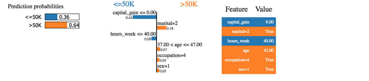
我们可以看到分类器正确地预测了这个家庭。收入确实高于 50k。
我们可以说的第一件事是,分类器对预测概率不是那么确定。该模型以 64% 的概率预测该家庭的收入超过 50k。这个 64% 由资本收益和婚姻状况组成。蓝色表示对正类有负贡献,橙色线表示有正贡献。
分类器之所以感到困惑,是因为这个家庭的资本收益为零,而资本收益通常是财富的一个良好预测指标。此外,该家庭每周工作时间少于 40 小时。年龄、职业和性别对分类器有积极贡献。
如果婚姻状况是单身,分类器将预测收入低于 50k (0.64-0.18 = 0.46)。
我们可以尝试另一个被错误分类的家庭。
temp.head(3)
temp.iloc[1,:-2]
age                  58
workclass             4
fnlwgt            68624
education            11
education_num         9
marital               2
occupation            4
relationship          0
race                  4
sex                   1
capital_gain          0
capital_loss          0
hours_week           45
native_country       38
Name: 20931, dtype: object
i = 1
print('This observation is', temp.iloc[i,-2:])
This observation is label        <=50K
predicted     >50K
Name: 20931, dtype: object
exp = explainer.explain_instance(temp.iloc[1,:-2], predict_fn, num_features=6)
exp.show_in_notebook(show_all=False)
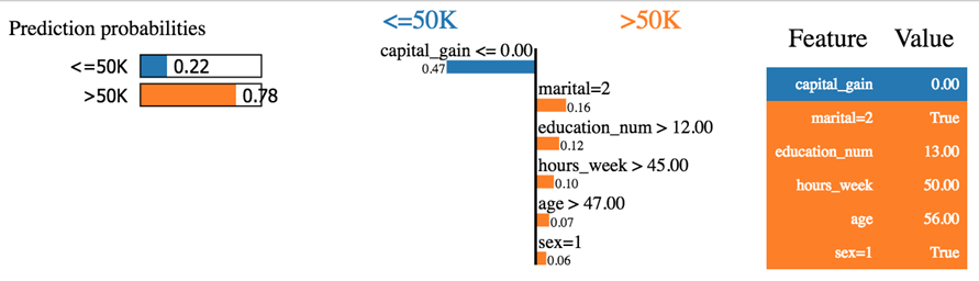
分类器预测收入低于 50k,但实际上并非如此。这个家庭看起来很奇怪。它没有资本收益,也没有资本损失。他已离婚,60 岁,受过良好教育,即 education_num > 12。根据整体模式,这个家庭应该像分类器所解释的那样,收入低于 50k。
您尝试玩弄 LIME。您会注意到分类器存在一些明显的错误。
您可以查看该库所有者的 GitHub。他们为图像和文本分类提供了额外的文档。
摘要
以下是一些适用于 scikit learn 版本 >=0.20 的有用命令列表:
| 创建训练/测试数据集 | 训练集拆分 |
| 构建管道 | |
| 选择列并应用转换 | makecolumntransformer |
| 转换类型 | |
| 标准化 | StandardScaler |
| 最小-最大标准化 | MinMaxScaler |
| 归一化 | Normalizer |
| 填充缺失值 | Imputer |
| 转换分类变量 | OneHotEncoder |
| 拟合和转换数据 | fit_transform |
| 创建管道 | make_pipeline |
| 基本模型 | |
| 逻辑回归 | LogisticRegression |
| XGBoost | XGBClassifier |
| 神经网络 | MLPClassifier |
| 网格搜索 | GridSearchCV |
| 随机搜索 | RandomizedSearchCV |