PySpark 初学者教程:通过示例学习
在学习 PySpark 之前,让我们先了解一下
什么是 Apache Spark?
Spark 是一种大数据解决方案,被证明比 Hadoop MapReduce 更简单、更快。Spark 是 UC Berkeley RAD lab 于 2009 年开发的一个开源软件。自 2010 年向公众发布以来,Spark 的受欢迎程度不断提高,并以前所未有的规模在行业中得到应用。
在大数据时代,从业者比以往任何时候都更需要快速可靠的工具来处理数据流。MapReduce 等早期工具很受欢迎,但速度很慢。为了解决这个问题,Spark 提供了一种既快速又通用的解决方案。Spark 与 MapReduce 的主要区别在于 Spark 在内存中进行计算,而 MapReduce 则在硬盘上进行计算。它允许高速访问和数据处理,将处理时间从几小时缩短到几分钟。
什么是 PySpark?
PySpark 是 Apache Spark 社区为将 Python 与 Spark 结合使用而创建的工具。它允许使用 Python 处理 RDD(弹性分布式数据集)。它还提供了 PySpark Shell,用于将 Python API 与 Spark Core 连接以启动 Spark Context。Spark 是实现集群计算的引擎名称,而 PySpark 是用于使用 Spark 的 Python 库。
Spark 如何工作?
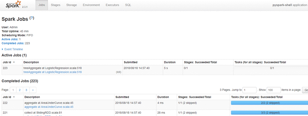
Spark 基于计算引擎,这意味着它负责应用程序的调度、分发和监控。每项任务都跨多个工作节点(称为计算集群)进行。计算集群是指任务的划分。一台机器执行一项任务,而其他机器通过不同的任务为最终输出做出贡献。最后,所有任务被聚合以产生输出。Spark 管理员提供对各种 Spark 作业的 360 度概述。
Spark 的设计目的是与
- Python
- Java
- Scala
- SQL
Spark 的一个显著特点是拥有大量内置库,包括用于机器学习的 MLlib。Spark 还设计用于与 Hadoop 集群配合使用,并且可以读取多种类型的文件,包括 Hive 数据、CSV、JSON、Cassandra 数据等。
为什么使用 Spark?
作为未来的数据从业者,您应该熟悉 Python 中流行的库:Pandas 和 scikit-learn。这两个库非常适合处理中小型数据集。常规的机器学习项目围绕以下方法论构建:
- 将数据加载到磁盘
- 将数据导入机器内存
- 处理/分析数据
- 构建机器学习模型
- 将预测结果存储回磁盘
如果数据科学家想处理的数据量太大,无法在一台计算机上完成,问题就出现了。在数据科学的早期,从业者会进行数据采样,因为处理大型数据集并非总是必需的。数据科学家会找到一个好的统计样本,进行额外的稳健性检查,并得出一个优秀的模型。
然而,这存在一些问题:
- 数据集是否反映了真实世界?
- 数据是否包含特定示例?
- 模型是否适合抽样?
以用户推荐为例。推荐系统依赖于将用户与其他用户进行比较来评估他们的偏好。如果数据从业者只选取数据的一个子集,就不会有与彼此非常相似的用户群体。推荐系统需要基于完整数据集运行,否则就无法运行。
解决方案是什么?
解决方案早已显而易见:将问题分解到多台计算机上。并行计算本身也带来多个问题。开发人员通常在编写并行代码时遇到困难,并最终不得不解决多处理本身带来的许多复杂问题。
Pyspark 为数据科学家提供了一个 API,可用于解决并行数据处理问题。Pyspark 处理多处理的复杂性,例如在机器集群上分发数据、分发代码以及收集工作人员的输出。
Spark 可以独立运行,但大多数情况下运行在 Hadoop 等集群计算框架之上。然而,在测试和开发中,数据科学家可以在他们的开发机或笔记本电脑上高效地运行 Spark,而无需集群。
• Spark 的主要优势之一是构建一个包含数据流管理、无缝数据查询、机器学习预测和对各种分析的实时访问的架构。
• Spark 与 SQL 语言紧密协作,即结构化数据。它允许实时查询数据。
• 数据科学家的主要工作是分析和构建预测模型。简而言之,数据科学家需要知道如何使用 SQL 查询数据、生成统计报告以及利用机器学习进行预测。数据科学家花费大量时间清理、转换和分析数据。一旦数据集或数据工作流准备就绪,数据科学家就会使用各种技术来发现见解和隐藏的模式。数据操作应该是健壮的,并且易于使用。Spark 因其速度和丰富的 API 而成为正确的工具。
在本 PySpark 教程中,您将学习如何使用 PySpark 示例构建分类器。
如何使用 AWS 安装 PySpark
Jupyter 团队构建了一个 Docker 镜像以高效运行 Spark。以下是您可以在 AWS 中安装 PySpark 实例的步骤。
请参阅我们关于 AWS 和 TensorFlow 的教程
步骤 1:创建实例
首先,您需要创建一个实例。登录您的 AWS 账户并启动实例。您可以将存储增加到 15g,并使用与 TensorFlow 教程相同的安全组。
步骤 2:建立连接
建立连接并安装 Docker 容器。更多详情,请参阅 TensorFlow 的教程与 Docker。请注意,您需要进入正确的目录。
只需运行这些代码即可安装 Docker
sudo yum update -y
sudo yum install -y docker
sudo service docker start
sudo user-mod -a -G docker ec2-user
exit
步骤 3:重新建立连接并安装 Spark
重新建立连接后,您可以安装包含 PySpark 的镜像。
## Spark
docker run -v ~/work:/home/jovyan/work -d -p 8888:8888 jupyter/pyspark-notebook

## Allow preserving Jupyter notebook
sudo chown 1000 ~/work

## Install tree to see our working directory next
sudo yum install -y tree
步骤 4:打开 Jupyter
检查容器及其名称
docker ps
使用 `docker logs` 加上 Docker 名称启动 Docker。例如:`docker logs zealous_goldwasser`
在浏览器中打开 Jupyter。地址是 https://:8888/。粘贴终端提供的密码。
注意:如果您想上传/下载文件到您的 AWS 机器,可以使用 Cyberduck 软件,https://cyberduck.io/。
如何使用 Conda 在 Windows/Mac 上安装 PySpark
以下是有关如何在 Windows/Mac 上使用 Anaconda 安装 PySpark 的详细过程
要在本地计算机上安装 Spark,推荐的做法是创建一个新的 conda 环境。这个新环境将安装 Python 3.6、Spark 以及所有依赖项。
Mac 用户
cd anaconda3
touch hello-spark.yml
vi hello-spark.yml
Windows 用户
cd C:\Users\Admin\Anaconda3
echo.>hello-spark.yml
notepad hello-spark.yml
您可以编辑 .yml 文件。请注意缩进。– 前需要两个空格
name: hello-spark
    dependencies:

    - python=3.6
    - jupyter
    - ipython
    - numpy
    - numpy-base
    - pandas
    - py4j
    - pyspark
    - pytz
保存并创建环境。这需要一些时间
conda env create -f hello-spark.yml
有关位置的更多详细信息,请参阅安装 TensorFlow 教程
您可以查看您机器上安装的所有环境
conda env list
Activate hello-spark
Mac 用户
source activate hello-spark
Windows 用户
activate hello-spark
注意:您已经创建了一个特定的 TensorFlow 环境来运行 TensorFlow 教程。将 Spark 或任何其他机器学习库添加到 hello-tf 环境中是没有意义的。最好创建一个与 hello-tf 不同的新环境。
设想您的项目大部分涉及 TensorFlow,但您只需要为某个特定项目使用 Spark。您可以为所有项目设置一个 TensorFlow 环境,并为 Spark 创建一个独立的环境。您可以在 Spark 环境中添加任意数量的库,而不会干扰 TensorFlow 环境。完成 Spark 项目后,您可以将其删除,而不会影响 TensorFlow 环境。
Jupyter
打开 Jupyter Notebook 并尝试 PySpark 是否正常工作。在新 Notebook 中粘贴以下 PySpark 示例代码:
import pyspark
from pyspark import SparkContext
sc =SparkContext()
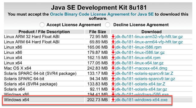
如果出现错误,很可能是您的机器上没有安装 Java。在 Mac 上,打开终端并输入 `java -version`,如果有 Java 版本,请确保它是 1.8。在 Windows 上,转到应用程序并检查是否有一个 Java 文件夹。如果有一个 Java 文件夹,请确保已安装 Java 1.8。截至本文撰写之时,PySpark 与 Java9 及更高版本不兼容。
如果您需要安装 Java,请访问此 链接 并下载 jdk-8u181-windows-x64.exe
对于 Mac 用户,建议使用 `brew`。
brew tap caskroom/versions
brew cask install java8
请参阅关于如何安装 Java 的分步教程
注意:使用 `remove` 可以完全删除一个环境。
conda env remove -n hello-spark -y
Spark Context
SparkContext 是允许与集群建立连接的内部引擎。如果您想运行一个操作,您需要一个 SparkContext。
创建 SparkContext
首先,您需要初始化一个 SparkContext。
import pyspark
from pyspark import SparkContext
sc =SparkContext()
现在 SparkContext 已准备就绪,您可以创建一个名为 RDD、弹性分布式数据集的数据集合。RDD 中的计算会自动并行化到整个集群。
nums= sc.parallelize([1,2,3,4])
您可以使用 `take` 访问第一行
nums.take(1)
[1]
您可以使用 lambda 函数对数据应用转换。在下面的 PySpark 示例中,您返回 `nums` 的平方。这是一个 map 转换。
squared = nums.map(lambda x: x*x).collect()
for num in squared:
    print('%i ' % (num))
1
4
9
16
SQLContext
更方便的方法是使用 DataFrame。SparkContext 已经设置好了,您可以使用它来创建 DataFrame。您还需要声明 SQLContext。
SQLContext 允许将引擎连接到不同的数据源。它用于初始化 Spark SQL 的功能。
from pyspark.sql import Row
from pyspark.sql import SQLContext

sqlContext = SQLContext(sc)
现在,在本 Spark 教程 Python 中,让我们创建一个包含姓名和年龄的元组列表。需要四个步骤:
步骤 1)用信息创建元组列表
[('John',19),('Smith',29),('Adam',35),('Henry',50)]
步骤 2)构建 RDD
rdd = sc.parallelize(list_p)
步骤 3)转换元组
rdd.map(lambda x: Row(name=x[0], age=int(x[1])))
步骤 4)创建 DataFrame 上下文
sqlContext.createDataFrame(ppl)
list_p = [('John',19),('Smith',29),('Adam',35),('Henry',50)]
rdd = sc.parallelize(list_p)
ppl = rdd.map(lambda x: Row(name=x[0], age=int(x[1])))
DF_ppl = sqlContext.createDataFrame(ppl)
如果您想访问每个特征的类型,您可以使用 `printSchema()`
DF_ppl.printSchema()
root
 |-- age: long (nullable = true)
 |-- name: string (nullable = true)
PySpark 机器学习示例
现在您对 Spark 和 SQLContext 有了初步了解,您就可以开始构建第一个机器学习程序了。
以下是使用 PySpark 构建机器学习程序的步骤:
- 步骤 1) PySpark 的基本操作
- 步骤 2)数据预处理
- 步骤 3)构建数据处理管道
- 步骤 4)构建分类器:逻辑回归
- 步骤 5)训练和评估模型
- 步骤 6)调整超参数
在本 PySpark 机器学习教程中,我们将使用 adult 数据集。本教程的目的是学习如何使用 Pyspark。有关数据集的更多信息,请参阅本教程。
请注意,数据集并不大,您可能会认为计算花费了很长时间。Spark 设计用于处理大量数据。当处理的数据集越大时,Spark 相对于其他机器学习库的性能就越高。
步骤 1) PySpark 的基本操作
首先,您需要初始化 SQLContext,如果尚未初始化的话。
#from pyspark.sql import SQLContext
url = "https://raw.githubusercontent.com/guru99-edu/R-Programming/master/adult_data.csv"
from pyspark import SparkFiles
sc.addFile(url)
sqlContext = SQLContext(sc)
然后,您可以使用 `sqlContext.read.csv` 读取 csv 文件。将 `inferSchema` 设置为 `True` 是为了让 Spark 自动猜测数据类型。默认情况下,它设置为 `False`。
df = sqlContext.read.csv(SparkFiles.get("adult_data.csv"), header=True, inferSchema= True)
让我们看一下数据类型
df.printSchema()
root
 |-- age: integer (nullable = true)
 |-- workclass: string (nullable = true)
 |-- fnlwgt: integer (nullable = true)
 |-- education: string (nullable = true)
 |-- education_num: integer (nullable = true)
 |-- marital: string (nullable = true)
 |-- occupation: string (nullable = true)
 |-- relationship: string (nullable = true)
 |-- race: string (nullable = true)
 |-- sex: string (nullable = true)
 |-- capital_gain: integer (nullable = true)
 |-- capital_loss: integer (nullable = true)
 |-- hours_week: integer (nullable = true)
 |-- native_country: string (nullable = true)
 |-- label: string (nullable = true)
您可以使用 `show` 查看数据。
df.show(5, truncate = False)
+---+----------------+------+---------+-------------+------------------+-----------------+-------------+-----+------+------------+------------+----------+--------------+-----+
|age|workclass       |fnlwgt|education|education_num|marital           |occupation       |relationship |race |sex   |capital_gain|capital_loss|hours_week|native_country|label|
+---+----------------+------+---------+-------------+------------------+-----------------+-------------+-----+------+------------+------------+----------+--------------+-----+
|39 |State-gov       |77516 |Bachelors|13           |Never-married     |Adm-clerical     |Not-in-family|White|Male  |2174        |0           |40        |United-States |<=50K|
|50 |Self-emp-not-inc|83311 |Bachelors|13           |Married-civ-spouse|Exec-managerial  |Husband      |White|Male  |0           |0           |13        |United-States |<=50K|
|38 |Private         |215646|HS-grad  |9            |Divorced          |Handlers-cleaners|Not-in-family|White|Male  |0           |0           |40        |United-States |<=50K|
|53 |Private         |234721|11th     |7            |Married-civ-spouse|Handlers-cleaners|Husband      |Black|Male  |0           |0           |40        |United-States |<=50K|
|28 |Private         |338409|Bachelors|13           |Married-civ-spouse|Prof-specialty   |Wife         |Black|Female|0           |0           |40        |Cuba          |<=50K|
+---+----------------+------+---------+-------------+------------------+-----------------+-------------+-----+------+------------+------------+----------+--------------+-----+
only showing top 5 rows
如果您没有将 `inferSchema` 设置为 `True`,就会发生这种情况。所有数据类型都将是字符串。
df_string = sqlContext.read.csv(SparkFiles.get("adult.csv"), header=True, inferSchema=  False)
df_string.printSchema()
root
 |-- age: string (nullable = true)
 |-- workclass: string (nullable = true)
 |-- fnlwgt: string (nullable = true)
 |-- education: string (nullable = true)
 |-- education_num: string (nullable = true)
 |-- marital: string (nullable = true)
 |-- occupation: string (nullable = true)
 |-- relationship: string (nullable = true)
 |-- race: string (nullable = true)
 |-- sex: string (nullable = true)
 |-- capital_gain: string (nullable = true)
 |-- capital_loss: string (nullable = true)
 |-- hours_week: string (nullable = true)
 |-- native_country: string (nullable = true)
 |-- label: string (nullable = true)
要将连续变量转换为正确的格式,您可以使用重新类型转换列。您可以使用 `withColumn` 来告诉 Spark 对哪些列执行转换。
# Import all from `sql.types`
from pyspark.sql.types import *

# Write a custom function to convert the data type of DataFrame columns
def convertColumn(df, names, newType):
    for name in names:
        df = df.withColumn(name, df[name].cast(newType))
    return df
# List of continuous features
CONTI_FEATURES  = ['age', 'fnlwgt','capital_gain', 'education_num', 'capital_loss', 'hours_week']
# Convert the type
df_string = convertColumn(df_string, CONTI_FEATURES, FloatType())
# Check the dataset
df_string.printSchema()
root
 |-- age: float (nullable = true)
 |-- workclass: string (nullable = true)
 |-- fnlwgt: float (nullable = true)
 |-- education: string (nullable = true)
 |-- education_num: float (nullable = true)
 |-- marital: string (nullable = true)
 |-- occupation: string (nullable = true)
 |-- relationship: string (nullable = true)
 |-- race: string (nullable = true)
 |-- sex: string (nullable = true)
 |-- capital_gain: float (nullable = true)
 |-- capital_loss: float (nullable = true)
 |-- hours_week: float (nullable = true)
 |-- native_country: string (nullable = true)
 |-- label: string (nullable = true)

from pyspark.ml.feature import StringIndexer
#stringIndexer = StringIndexer(inputCol="label", outputCol="newlabel")
#model = stringIndexer.fit(df)
#df = model.transform(df)
df.printSchema()
选择列
您可以使用 `select` 和特征名称来选择并显示行。下面选择了 `age` 和 `fnlwgt`。
df.select('age','fnlwgt').show(5)
+---+------+
|age|fnlwgt|
+---+------+
| 39| 77516|
| 50| 83311|
| 38|215646|
| 53|234721|
| 28|338409|
+---+------+
only showing top 5 rows
按组计数
如果您想计算每个组的出现次数,可以链式调用
- groupBy()
- count()
在一起来。在下面的 PySpark 示例中,您将按教育水平计数行数。
df.groupBy("education").count().sort("count",ascending=True).show()
+------------+-----+
|   education|count|
+------------+-----+
|   Preschool|   51|
|     1st-4th|  168|
|     5th-6th|  333|
|   Doctorate|  413|
|        12th|  433|
|         9th|  514|
| Prof-school|  576|
|     7th-8th|  646|
|        10th|  933|
|  Assoc-acdm| 1067|
|        11th| 1175|
|   Assoc-voc| 1382|
|     Masters| 1723|
|   Bachelors| 5355|
|Some-college| 7291|
|     HS-grad|10501|
+------------+-----+
描述数据
要获取数据的摘要统计信息,您可以使用 `describe()`。它将计算
- 计数
- 平均值
- 标准差
- min
- max
df.describe().show()
+-------+------------------+-----------+------------------+------------+-----------------+--------+----------------+------------+------------------+------+------------------+----------------+------------------+--------------+-----+
|summary|               age|  workclass|            fnlwgt|   education|    education_num| marital|      occupation|relationship|              race|   sex|      capital_gain|    capital_loss|        hours_week|native_country|label|
+-------+------------------+-----------+------------------+------------+-----------------+--------+----------------+------------+------------------+------+------------------+----------------+------------------+--------------+-----+
|  count|             32561|      32561|             32561|       32561|            32561|   32561|           32561|       32561|             32561| 32561|             32561|           32561|             32561|         32561|32561|
|   mean| 38.58164675532078|       null|189778.36651208502|        null| 10.0806793403151|    null|            null|        null|              null|  null|1077.6488437087312| 87.303829734959|40.437455852092995|          null| null|
| stddev|13.640432553581356|       null|105549.97769702227|        null|2.572720332067397|    null|            null|        null|              null|  null| 7385.292084840354|402.960218649002|12.347428681731838|          null| null|
|    min|                17|          ?|             12285|        10th|                1|Divorced|               ?|     Husband|Amer-Indian-Eskimo|Female|                 0|               0|                 1|             ?|<=50K|
|    max|                90|Without-pay|           1484705|Some-college|               16| Widowed|Transport-moving|        Wife|             White|  Male|             99999|            4356|                99|    Yugoslavia| >50K|
+-------+------------------+-----------+------------------+------------+-----------------+--------+----------------+------------+------------------+------+------------------+----------------+------------------+--------------+-----+
如果您只想获取一列的摘要统计信息,请在 `describe()` 中添加列名。
df.describe('capital_gain').show()
+-------+------------------+
|summary|      capital_gain|
+-------+------------------+
|  count|             32561|
|   mean|1077.6488437087312|
| stddev| 7385.292084840354|
|    min|                 0|
|    max|             99999|
+-------+------------------+
交叉表计算
在某些情况下,了解两个配对列之间的描述性统计信息会很有用。例如,您可以按教育水平计算收入低于或高于 50k 的人数。此操作称为交叉表。
df.crosstab('age', 'label').sort("age_label").show()
+---------+-----+----+
|age_label|<=50K|>50K|
+---------+-----+----+
|       17|  395|   0|
|       18|  550|   0|
|       19|  710|   2|
|       20|  753|   0|
|       21|  717|   3|
|       22|  752|  13|
|       23|  865|  12|
|       24|  767|  31|
|       25|  788|  53|
|       26|  722|  63|
|       27|  754|  81|
|       28|  748| 119|
|       29|  679| 134|
|       30|  690| 171|
|       31|  705| 183|
|       32|  639| 189|
|       33|  684| 191|
|       34|  643| 243|
|       35|  659| 217|
|       36|  635| 263|
+---------+-----+----+
only showing top 20 rows
您可以看到,当人们年轻时,很少有人收入超过 50k。
删除列
有两个直观的 API 可以删除列:
- drop(): 删除一列
- dropna(): 删除 NA 值
下面我们删除 `education_num` 列。
df.drop('education_num').columns

['age',
 'workclass',
 'fnlwgt',
 'education',
 'marital',
 'occupation',
 'relationship',
 'race',
 'sex',
 'capital_gain',
 'capital_loss',
 'hours_week',
 'native_country',
 'label']
过滤数据
您可以使用 `filter()` 对数据子集应用描述性统计。例如,您可以计算 40 岁以上的人数。
df.filter(df.age > 40).count()
13443
按组的描述性统计
最后,您可以按组对数据进行分组,并计算平均值等统计运算。
df.groupby('marital').agg({'capital_gain': 'mean'}).show()
+--------------------+------------------+
|             marital| avg(capital_gain)|
+--------------------+------------------+
|           Separated| 535.5687804878049|
|       Never-married|376.58831788823363|
|Married-spouse-ab...| 653.9832535885167|
|            Divorced| 728.4148098131893|
|             Widowed| 571.0715005035247|
|   Married-AF-spouse| 432.6521739130435|
|  Married-civ-spouse|1764.8595085470085|
+--------------------+------------------+
步骤 2) 数据预处理
数据处理是机器学习中的关键步骤。在您删除垃圾数据后,您会获得一些重要的见解。
例如,您知道年龄与收入不是线性关系。当人们年轻时,他们的收入通常低于中年。退休后,家庭会使用他们的储蓄,这意味着收入会下降。为了捕捉这种模式,您可以为年龄特征添加平方项。
添加年龄平方
要添加一个新特征,您需要
- 选择列
- 应用转换并将其添加到 DataFrame
from pyspark.sql.functions import *

# 1 Select the column
age_square = df.select(col("age")**2)

# 2 Apply the transformation and add it to the DataFrame
df = df.withColumn("age_square", col("age")**2)

df.printSchema()
root
 |-- age: integer (nullable = true)
 |-- workclass: string (nullable = true)
 |-- fnlwgt: integer (nullable = true)
 |-- education: string (nullable = true)
 |-- education_num: integer (nullable = true)
 |-- marital: string (nullable = true)
 |-- occupation: string (nullable = true)
 |-- relationship: string (nullable = true)
 |-- race: string (nullable = true)
 |-- sex: string (nullable = true)
 |-- capital_gain: integer (nullable = true)
 |-- capital_loss: integer (nullable = true)
 |-- hours_week: integer (nullable = true)
 |-- native_country: string (nullable = true)
 |-- label: string (nullable = true)
 |-- age_square: double (nullable = true)
您可以看到 `age_square` 已成功添加到 DataFrame 中。您可以使用 `select` 更改变量的顺序。下面,我们将 `age_square` 放在 `age` 之后。
COLUMNS = ['age', 'age_square', 'workclass', 'fnlwgt', 'education', 'education_num', 'marital',
           'occupation', 'relationship', 'race', 'sex', 'capital_gain', 'capital_loss',
           'hours_week', 'native_country', 'label']
df = df.select(COLUMNS)
df.first()
Row(age=39, age_square=1521.0, workclass='State-gov', fnlwgt=77516, education='Bachelors', education_num=13, marital='Never-married', occupation='Adm-clerical', relationship='Not-in-family', race='White', sex='Male', capital_gain=2174, capital_loss=0, hours_week=40, native_country='United-States', label='<=50K')
排除荷兰-荷兰
当一个特征中的一个组只有一个观测值时,它不会为模型提供信息。相反,它可能导致交叉验证期间出错。
让我们检查一下家庭的来源
df.filter(df.native_country == 'Holand-Netherlands').count()
df.groupby('native_country').agg({'native_country': 'count'}).sort(asc("count(native_country)")).show()
+--------------------+---------------------+
|      native_country|count(native_country)|
+--------------------+---------------------+
|  Holand-Netherlands|                    1|
|            Scotland|                   12|
|             Hungary|                   13|
|            Honduras|                   13|
|Outlying-US(Guam-...|                   14|
|          Yugoslavia|                   16|
|            Thailand|                   18|
|                Laos|                   18|
|            Cambodia|                   19|
|     Trinadad&Tobago|                   19|
|                Hong|                   20|
|             Ireland|                   24|
|             Ecuador|                   28|
|              Greece|                   29|
|              France|                   29|
|                Peru|                   31|
|           Nicaragua|                   34|
|            Portugal|                   37|
|                Iran|                   43|
|               Haiti|                   44|
+--------------------+---------------------+
only showing top 20 rows
特征 `native_country` 只有一个来自荷兰的家庭。您将其排除。
df_remove = df.filter(df.native_country != 'Holand-Netherlands')
步骤 3) 构建数据处理管道
与 scikit-learn 类似,Pyspark 也有一个管道 API。
管道非常方便地维护数据结构。您将数据推送到管道中。在管道内部,执行各种操作,输出用于馈送算法。
例如,机器学习中的一个通用转换是将字符串转换为独热编码(one-hot encoder),即每个组一个列。独热编码通常是一个全是零的矩阵。
转换数据的步骤与 scikit-learn 非常相似。您需要
- 索引字符串到数字
- 创建独热编码器
- 转换数据
有两个 API 可以完成这项工作:`StringIndexer`、`OneHotEncoder`
- 首先,您选择要索引的字符串列。`inputCol` 是数据集中列的名称。`outputCol` 是转换后的新列名。
StringIndexer(inputCol="workclass", outputCol="workclass_encoded")
- 拟合数据并进行转换
model = stringIndexer.fit(df)
`indexed = model.transform(df)``
- 基于组创建新列。例如,如果特征中有 10 个组,则新矩阵将有 10 列,每列代表一个组。
OneHotEncoder(dropLast=False, inputCol="workclassencoded", outputCol="workclassvec")
### Example encoder
from pyspark.ml.feature import StringIndexer, OneHotEncoder, VectorAssembler

stringIndexer = StringIndexer(inputCol="workclass", outputCol="workclass_encoded")
model = stringIndexer.fit(df)
indexed = model.transform(df)
encoder = OneHotEncoder(dropLast=False, inputCol="workclass_encoded", outputCol="workclass_vec")
encoded = encoder.transform(indexed)
encoded.show(2)
+---+----------+----------------+------+---------+-------------+------------------+---------------+-------------+-----+----+------------+------------+----------+--------------+-----+-----------------+-------------+
|age|age_square|       workclass|fnlwgt|education|education_num|           marital|     occupation| relationship| race| sex|capital_gain|capital_loss|hours_week|native_country|label|workclass_encoded|workclass_vec|
+---+----------+----------------+------+---------+-------------+------------------+---------------+-------------+-----+----+------------+------------+----------+--------------+-----+-----------------+-------------+
| 39|    1521.0|       State-gov| 77516|Bachelors|           13|     Never-married|   Adm-clerical|Not-in-family|White|Male|        2174|           0|        40| United-States|<=50K|              4.0|(9,[4],[1.0])|
| 50|    2500.0|Self-emp-not-inc| 83311|Bachelors|           13|Married-civ-spouse|Exec-managerial|      Husband|White|Male|           0|           0|        13| United-States|<=50K|              1.0|(9,[1],[1.0])|
+---+----------+----------------+------+---------+-------------+------------------+---------------+-------------+-----+----+------------+------------+----------+--------------+-----+-----------------+-------------+
only showing top 2 rows
构建管道
您将构建一个管道来转换所有精确的特征并将它们添加到最终数据集中。该管道将包含四种操作,但您可以随时添加更多操作。
- 编码分类数据
- 索引标签特征
- 添加连续变量
- 组装步骤。
每个步骤都存储在名为 `stages` 的列表中。此列表将告诉 `VectorAssembler` 在管道内执行什么操作。
1. 编码分类数据
此步骤与上面的示例完全相同,只是您遍历所有分类特征。
from pyspark.ml import Pipeline
from pyspark.ml.feature import OneHotEncoderEstimator
CATE_FEATURES = ['workclass', 'education', 'marital', 'occupation', 'relationship', 'race', 'sex', 'native_country']
stages = [] # stages in our Pipeline
for categoricalCol in CATE_FEATURES:
    stringIndexer = StringIndexer(inputCol=categoricalCol, outputCol=categoricalCol + "Index")
    encoder = OneHotEncoderEstimator(inputCols=[stringIndexer.getOutputCol()],
                                     outputCols=[categoricalCol + "classVec"])
    stages += [stringIndexer, encoder]
2. 索引标签特征
Spark 和许多其他库一样,不接受字符串值作为标签。您使用 `StringIndexer` 转换标签特征并将其添加到 `stages` 列表中。
# Convert label into label indices using the StringIndexer
label_stringIdx =  StringIndexer(inputCol="label", outputCol="newlabel")
stages += [label_stringIdx]
3. 添加连续变量
`VectorAssembler` 的 `inputCols` 是一个列列表。您可以创建一个新列表,其中包含所有新列。下面的代码将编码的分类特征和连续特征填充到列表中。
assemblerInputs = [c + "classVec" for c in CATE_FEATURES] + CONTI_FEATURES
4. 组装步骤。
最后,您将所有步骤传递给 `VectorAssembler`。
assembler = VectorAssembler(inputCols=assemblerInputs, outputCol="features")stages += [assembler]
现在所有步骤都已准备就绪,您将数据推送到管道。
# Create a Pipeline.
pipeline = Pipeline(stages=stages)
pipelineModel = pipeline.fit(df_remove)
model = pipelineModel.transform(df_remove)
如果您查看新数据集,您会发现它包含了所有特征,包括转换前和转换后的。您只对 `newlabel` 和 `features` 感兴趣。`features` 包括所有转换后的特征和连续变量。
model.take(1)

[Row(age=39, age_square=1521.0, workclass='State-gov', fnlwgt=77516, education='Bachelors', education_num=13, marital='Never-married', occupation='Adm-clerical', relationship='Not-in-family', race='White', sex='Male', capital_gain=2174, capital_loss=0, hours_week=40, native_country='United-States', label='<=50K', workclassIndex=4.0, workclassclassVec=SparseVector(8, {4: 1.0}), educationIndex=2.0, educationclassVec=SparseVector(15, {2: 1.0}), maritalIndex=1.0, maritalclassVec=SparseVector(6, {1: 1.0}), occupationIndex=3.0, occupationclassVec=SparseVector(14, {3: 1.0}), relationshipIndex=1.0, relationshipclassVec=SparseVector(5, {1: 1.0}), raceIndex=0.0, raceclassVec=SparseVector(4, {0: 1.0}), sexIndex=0.0, sexclassVec=SparseVector(1, {0: 1.0}), native_countryIndex=0.0, native_countryclassVec=SparseVector(40, {0: 1.0}), newlabel=0.0, features=SparseVector(99, {4: 1.0, 10: 1.0, 24: 1.0, 32: 1.0, 44: 1.0, 48: 1.0, 52: 1.0, 53: 1.0, 93: 39.0, 94: 77516.0, 95: 2174.0, 96: 13.0, 98: 40.0}))]
步骤 4) 构建分类器:逻辑回归
为了加快计算速度,您可以将模型转换为 DataFrame。
您需要使用 `map` 从模型中选择 `newlabel` 和 `features`。
from pyspark.ml.linalg import DenseVector
input_data = model.rdd.map(lambda x: (x["newlabel"], DenseVector(x["features"])))
您可以使用 `sqlContext` 创建训练数据 DataFrame。
df_train = sqlContext.createDataFrame(input_data, ["label", "features"])
查看第二行
df_train.show(2)
+-----+--------------------+
|label|            features|
+-----+--------------------+
|  0.0|[0.0,0.0,0.0,0.0,...|
|  0.0|[0.0,1.0,0.0,0.0,...|
+-----+--------------------+
only showing top 2 rows
创建训练/测试集
您使用 `randomSplit` 将数据集分为 80/20。
# Split the data into train and test sets
train_data, test_data = df_train.randomSplit([.8,.2],seed=1234)
让我们计算训练集和测试集中收入低于/高于 50k 的人数。
train_data.groupby('label').agg({'label': 'count'}).show()
+-----+------------+
|label|count(label)|
+-----+------------+
|  0.0|       19698|
|  1.0|        6263|
+-----+------------+
test_data.groupby('label').agg({'label': 'count'}).show()
+-----+------------+
|label|count(label)|
+-----+------------+
|  0.0|        5021|
|  1.0|        1578|
+-----+------------+
构建逻辑回归器
最后但并非最不重要的一点是,您可以构建分类器。Pyspark 有一个名为 `LogisticRegression` 的 API 来执行逻辑回归。
您通过指定标签列和特征列来初始化 `lr`。您将最大迭代次数设置为 10,并添加一个值为 0.3 的正则化参数。请注意,在下一节中,您将使用具有参数网格的交叉验证来调整模型。
# Import `LinearRegression`
from pyspark.ml.classification import LogisticRegression

# Initialize `lr`
lr = LogisticRegression(labelCol="label",
                        featuresCol="features",
                        maxIter=10,
                        regParam=0.3)

# Fit the data to the model
linearModel = lr.fit(train_data)
# 您可以看到回归的系数
# Print the coefficients and intercept for logistic regression
print("Coefficients: " + str(linearModel.coefficients))
print("Intercept: " + str(linearModel.intercept))
Coefficients: [-0.0678914665262,-0.153425526813,-0.0706009536407,-0.164057586562,-0.120655298528,0.162922330862,0.149176870438,-0.626836362611,-0.193483661541,-0.0782269980838,0.222667203836,0.399571096381,-0.0222024341804,-0.311925857859,-0.0434497788688,-0.306007744328,-0.41318209688,0.547937504247,-0.395837350854,-0.23166535958,0.618743906733,-0.344088614546,-0.385266881369,0.317324463006,-0.350518889186,-0.201335923138,-0.232878560088,-0.13349278865,-0.119760542498,0.17500602491,-0.0480968101118,0.288484253943,-0.116314616745,0.0524163478063,-0.300952624551,-0.22046421474,-0.16557996579,-0.114676231939,-0.311966431453,-0.344226119233,0.105530129507,0.152243047814,-0.292774545497,0.263628334433,-0.199951374076,-0.30329422583,-0.231087515178,0.418918551,-0.0565930184279,-0.177818073048,-0.0733236680663,-0.267972912252,0.168491215697,-0.12181255723,-0.385648075442,-0.202101794517,0.0469791640782,-0.00842850210625,-0.00373211448629,-0.259296141281,-0.309896554133,-0.168434409756,-0.11048086026,0.0280647963877,-0.204187030092,-0.414392623536,-0.252806580669,0.143366465705,-0.516359222663,-0.435627370849,-0.301949286524,0.0878249035894,-0.210951740965,-0.621417928742,-0.099445190784,-0.232671473401,-0.1077745606,-0.360429419703,-0.420362959052,-0.379729467809,-0.395186242741,0.0826401853838,-0.280251589972,0.187313505214,-0.20295228799,-0.431177064626,0.149759018379,-0.107114299614,-0.319314858424,0.0028450133235,-0.651220387649,-0.327918792207,-0.143659581445,0.00691075160413,8.38517628783e-08,2.18856717378e-05,0.0266701216268,0.000231075966823,0.00893832698698]
Intercept: -1.9884177974805692
步骤 5) 训练和评估模型
要为您的测试集生成预测,
您可以在 `test_data` 上使用 `transform()` 来使用 `linearModel`。
# Make predictions on test data using the transform() method.
predictions = linearModel.transform(test_data)
您可以打印 `predictions` 中的元素。
predictions.printSchema()
root
 |-- label: double (nullable = true)
 |-- features: vector (nullable = true)
 |-- rawPrediction: vector (nullable = true)
 |-- probability: vector (nullable = true)
 |-- prediction: double (nullable = false)
您关心的是标签、预测和概率。
selected = predictions.select("label", "prediction", "probability")
selected.show(20)
+-----+----------+--------------------+
|label|prediction|         probability|
+-----+----------+--------------------+
|  0.0|       0.0|[0.91560704124179...|
|  0.0|       0.0|[0.92812140213994...|
|  0.0|       0.0|[0.92161406774159...|
|  0.0|       0.0|[0.96222760777142...|
|  0.0|       0.0|[0.66363283056957...|
|  0.0|       0.0|[0.65571324475477...|
|  0.0|       0.0|[0.73053376932829...|
|  0.0|       1.0|[0.31265053873570...|
|  0.0|       0.0|[0.80005907577390...|
|  0.0|       0.0|[0.76482251301640...|
|  0.0|       0.0|[0.84447301189069...|
|  0.0|       0.0|[0.75691912026619...|
|  0.0|       0.0|[0.60902504096722...|
|  0.0|       0.0|[0.80799228385509...|
|  0.0|       0.0|[0.87704364852567...|
|  0.0|       0.0|[0.83817652582377...|
|  0.0|       0.0|[0.79655423248500...|
|  0.0|       0.0|[0.82712311232246...|
|  0.0|       0.0|[0.81372823882016...|
|  0.0|       0.0|[0.59687710752201...|
+-----+----------+--------------------+
only showing top 20 rows
评估模型
您需要查看准确率指标来了解模型的性能如何(好或坏)。目前,Spark 中没有计算准确率的 API。默认值是 ROC(接收者操作特征曲线)。这是一个不同的指标,它考虑了假阳性率。这是一个不同的指标,它考虑了假阳性率。
在查看 ROC 之前,让我们构建准确率度量。您对这个度量更熟悉。准确率度量是正确预测数除以总观测数。
您创建一个包含标签和 `prediction` 的 DataFrame。
cm = predictions.select("label", "prediction")
您可以检查标签和预测中的类别数量。
cm.groupby('label').agg({'label': 'count'}).show()
+-----+------------+
|label|count(label)|
+-----+------------+
|  0.0|        5021|
|  1.0|        1578|
+-----+------------+
cm.groupby('prediction').agg({'prediction': 'count'}).show()
+----------+-----------------+
|prediction|count(prediction)|
+----------+-----------------+
|       0.0|             5982|
|       1.0|              617|
+----------+-----------------+
例如,在测试集中,有 1578 个家庭的收入高于 50k,有 5021 个家庭低于 50k。然而,分类器预测有 617 个家庭的收入高于 50k。
您可以通过计算正确分类标签的计数除以总行数来计算准确率。
cm.filter(cm.label == cm.prediction).count() / cm.count()
0.8237611759357478
您可以将所有内容包装在一起并编写一个函数来计算准确率。
def accuracy_m(model):
    predictions = model.transform(test_data)
    cm = predictions.select("label", "prediction")
    acc = cm.filter(cm.label == cm.prediction).count() / cm.count()
    print("Model accuracy: %.3f%%" % (acc * 100))
accuracy_m(model = linearModel)
Model accuracy: 82.376%
ROC 指标
模块 `BinaryClassificationEvaluator` 包含 ROC 度量。接收者操作特征曲线是二分类中另一个常用的工具。它与精确率/召回率曲线非常相似,但它不是绘制精确率与召回率,而是 ROC 曲线显示真阳性率(即召回率)与假阳性率。假阳性率是指被错误地分类为阳性的阴性实例的比例。它等于 1 减去真阴性率。真阴性率也称为特异度。因此,ROC 曲线绘制敏感性(召回率)与 1 – 特异度。
### Use ROC
from pyspark.ml.evaluation import BinaryClassificationEvaluator

# Evaluate model
evaluator = BinaryClassificationEvaluator(rawPredictionCol="rawPrediction")
print(evaluator.evaluate(predictions))
print(evaluator.getMetricName())
0.8940481662695192 曲线下面积
print(evaluator.evaluate(predictions))
0.8940481662695192
步骤 6) 调整超参数
最后但并非最不重要的一点是,您可以调整超参数。与 scikit learn 类似,您可以创建一个参数网格,并添加您要调整的参数。
为了缩短计算时间,您只用两个值来调整正则化参数。
from pyspark.ml.tuning import ParamGridBuilder, CrossValidator

# Create ParamGrid for Cross Validation
paramGrid = (ParamGridBuilder()
             .addGrid(lr.regParam, [0.01, 0.5])
             .build())
最后,您使用 5 折交叉验证来评估模型。训练大约需要 16 分钟。
from time import *
start_time = time()

# Create 5-fold CrossValidator
cv = CrossValidator(estimator=lr,
                    estimatorParamMaps=paramGrid,
                    evaluator=evaluator, numFolds=5)

# Run cross validations
cvModel = cv.fit(train_data)
# likely take a fair amount of time
end_time = time()
elapsed_time = end_time - start_time
print("Time to train model: %.3f seconds" % elapsed_time)
模型训练时间:978.807 秒
最佳正则化超参数是 0.01,准确率为 85.316%。
accuracy_m(model = cvModel)
Model accuracy: 85.316%
您可以通过链接 `cvModel.bestModel` 和 `extractParamMap()` 来提取推荐的参数。
bestModel = cvModel.bestModel
bestModel.extractParamMap()
{Param(parent='LogisticRegression_4d8f8ce4d6a02d8c29a0', name='aggregationDepth', doc='suggested depth for treeAggregate (>= 2)'): 2,
 Param(parent='LogisticRegression_4d8f8ce4d6a02d8c29a0', name='elasticNetParam', doc='the ElasticNet mixing parameter, in range [0, 1]. For alpha = 0, the penalty is an L2 penalty. For alpha = 1, it is an L1 penalty'): 0.0,
 Param(parent='LogisticRegression_4d8f8ce4d6a02d8c29a0', name='family', doc='The name of family which is a description of the label distribution to be used in the model. Supported options: auto, binomial, multinomial.'): 'auto',
 Param(parent='LogisticRegression_4d8f8ce4d6a02d8c29a0', name='featuresCol', doc='features column name'): 'features',
 Param(parent='LogisticRegression_4d8f8ce4d6a02d8c29a0', name='fitIntercept', doc='whether to fit an intercept term'): True,
 Param(parent='LogisticRegression_4d8f8ce4d6a02d8c29a0', name='labelCol', doc='label column name'): 'label',
 Param(parent='LogisticRegression_4d8f8ce4d6a02d8c29a0', name='maxIter', doc='maximum number of iterations (>= 0)'): 10,
 Param(parent='LogisticRegression_4d8f8ce4d6a02d8c29a0', name='predictionCol', doc='prediction column name'): 'prediction',
 Param(parent='LogisticRegression_4d8f8ce4d6a02d8c29a0', name='probabilityCol', doc='Column name for predicted class conditional probabilities. Note: Not all models output well-calibrated probability estimates! These probabilities should be treated as confidences, not precise probabilities'): 'probability',
 Param(parent='LogisticRegression_4d8f8ce4d6a02d8c29a0', name='rawPredictionCol', doc='raw prediction (a.k.a. confidence) column name'): 'rawPrediction',
 Param(parent='LogisticRegression_4d8f8ce4d6a02d8c29a0', name='regParam', doc='regularization parameter (>= 0)'): 0.01,
 Param(parent='LogisticRegression_4d8f8ce4d6a02d8c29a0', name='standardization', doc='whether to standardize the training features before fitting the model'): True,
 Param(parent='LogisticRegression_4d8f8ce4d6a02d8c29a0', name='threshold', doc='threshold in binary classification prediction, in range [0, 1]'): 0.5,
 Param(parent='LogisticRegression_4d8f8ce4d6a02d8c29a0', name='tol', doc='the convergence tolerance for iterative algorithms (>= 0)'): 1e-06}
摘要
Spark 是数据科学家的基本工具。它允许从业者将应用程序连接到不同的数据源,无缝地执行数据分析或添加预测模型。
要开始使用 Spark,您需要初始化一个 Spark Context
‘SparkContext()’
和一个 SQL Context 来连接到数据源
‘SQLContext()’
在本教程中,您将学习如何训练逻辑回归模型
- 使用以下方法将数据集转换为 DataFrame:
rdd.map(lambda x: (x["newlabel"], DenseVector(x["features"])))
sqlContext.createDataFrame(input_data, ["label", "features"])
请注意,标签的列名为 `newlabel`,所有特征都收集在 `features` 中。如果您的数据集中这些名称不同,请进行相应更改。
- 创建训练/测试集
randomSplit([.8,.2],seed=1234)
- 训练模型
LogisticRegression(labelCol="label",featuresCol="features",maxIter=10, regParam=0.3)
lr.fit()
- 进行预测
linearModel.transform()