R中的决策树:带示例的分类树
什么是决策树?
决策树是一种多功能的机器学习算法,可以执行分类和回归任务。它们是非常强大的算法,能够拟合复杂的数据集。此外,决策树是随机森林的基本组成部分,而随机森林是当今最强大的机器学习算法之一。
在 R 中训练和可视化决策树
为了在 R 示例中构建你的第一个决策树,我们将按照此决策树教程中的步骤进行:
- 步骤1: 导入数据
- 步骤 2:清理数据集
- 步骤 3:创建训练/测试集
- 步骤 4:构建模型
- 步骤 5:进行预测
- 步骤 6:评估性能
- 步骤 7:调整超参数
步骤 1) 导入数据
如果你对泰坦尼克号的命运感到好奇,可以观看这个 Youtube 视频。该数据集的目的是预测哪些人在与冰山碰撞后更有可能生存下来。该数据集包含 13 个变量和 1309 个观测值。数据集按变量 X 排序。
set.seed(678)
path <- 'https://raw.githubusercontent.com/guru99-edu/R-Programming/master/titanic_data.csv'
titanic <-read.csv(path)
head(titanic)
输出
##   X pclass survived                                            name    sex
## 1 1      1        1                   Allen, Miss. Elisabeth Walton female
## 2 2      1        1                  Allison, Master. Hudson Trevor   male
## 3 3      1        0                    Allison, Miss. Helen Loraine female
## 4 4      1        0            Allison, Mr. Hudson Joshua Creighton   male
## 5 5      1        0 Allison, Mrs. Hudson J C (Bessie Waldo Daniels) female
## 6 6      1        1                             Anderson, Mr. Harry   male
##       age sibsp parch ticket     fare   cabin embarked
## 1 29.0000     0     0  24160 211.3375      B5        S
## 2  0.9167     1     2 113781 151.5500 C22 C26        S
## 3  2.0000     1     2 113781 151.5500 C22 C26        S
## 4 30.0000     1     2 113781 151.5500 C22 C26        S
## 5 25.0000     1     2 113781 151.5500 C22 C26        S
## 6 48.0000     0     0  19952  26.5500     E12        S
##                         home.dest
## 1                    St Louis, MO
## 2 Montreal, PQ / Chesterville, ON
## 3 Montreal, PQ / Chesterville, ON
## 4 Montreal, PQ / Chesterville, ON
## 5 Montreal, PQ / Chesterville, ON
## 6                    New York, NY
tail(titanic)
输出
##         X pclass survived                      name    sex  age sibsp
## 1304 1304      3        0     Yousseff, Mr. Gerious   male   NA     0
## 1305 1305      3        0      Zabour, Miss. Hileni female 14.5     1
## 1306 1306      3        0     Zabour, Miss. Thamine female   NA     1
## 1307 1307      3        0 Zakarian, Mr. Mapriededer   male 26.5     0
## 1308 1308      3        0       Zakarian, Mr. Ortin   male 27.0     0
## 1309 1309      3        0        Zimmerman, Mr. Leo   male 29.0     0
##      parch ticket    fare cabin embarked home.dest
## 1304     0   2627 14.4583              C
## 1305     0   2665 14.4542              C
## 1306     0   2665 14.4542              C
## 1307     0   2656  7.2250              C
## 1308     0   2670  7.2250              C
## 1309     0 315082  7.8750              S
从 head 和 tail 的输出中,你可以注意到数据没有被打乱。这是一个大问题!当你将数据拆分为训练集和测试集时,你将只选择来自头等舱和二等舱的乘客(前 80% 的观测值中没有三等舱的乘客),这意味着算法将永远看不到三等舱乘客的特征。这个错误将导致预测性能不佳。
要解决这个问题,你可以使用 sample() 函数。
shuffle_index <- sample(1:nrow(titanic))
head(shuffle_index)
决策树 R 代码解释
- sample(1:nrow(titanic)):生成一个从 1 到 1309(即最大行数)的随机索引列表。
输出
## [1] 288 874 1078 633 887 992
你将使用此索引来打乱 titanic 数据集。
titanic <- titanic[shuffle_index, ]
head(titanic)
输出
##         X pclass survived
## 288   288      1        0
## 874   874      3        0
## 1078 1078      3        1
## 633   633      3        0
## 887   887      3        1
## 992   992      3        1
##                                                           name    sex age
## 288                                      Sutton, Mr. Frederick   male  61
## 874                   Humblen, Mr. Adolf Mathias Nicolai Olsen   male  42
## 1078                                 O'Driscoll, Miss. Bridget female  NA
## 633  Andersson, Mrs. Anders Johan (Alfrida Konstantia Brogren) female  39
## 887                                        Jermyn, Miss. Annie female  NA
## 992                                           Mamee, Mr. Hanna   male  NA
##      sibsp parch ticket    fare cabin embarked           home.dest## 288      0     0  36963 32.3208   D50        S     Haddenfield, NJ
## 874      0     0 348121  7.6500 F G63        S
## 1078     0     0  14311  7.7500              Q
## 633      1     5 347082 31.2750              S Sweden Winnipeg, MN
## 887      0     0  14313  7.7500              Q
## 992      0     0   2677  7.2292              C
步骤 2) 清理数据集
数据结构显示某些变量具有 NA。数据清理步骤如下:
- 删除变量 home.dest、cabin、name、X 和 ticket
- 为 pclass 和 survived 创建因子变量
- 删除 NA
library(dplyr)
# Drop variables
clean_titanic <- titanic % > %
select(-c(home.dest, cabin, name, X, ticket)) % > %
#Convert to factor level
	mutate(pclass = factor(pclass, levels = c(1, 2, 3), labels = c('Upper', 'Middle', 'Lower')),
	survived = factor(survived, levels = c(0, 1), labels = c('No', 'Yes'))) % > %
na.omit()
glimpse(clean_titanic)
代码解释
- select(-c(home.dest, cabin, name, X, ticket)):删除不必要的变量。
- pclass = factor(pclass, levels = c(1,2,3), labels= c(‘Upper’, ‘Middle’, ‘Lower’)):为 pclass 变量添加标签。1 变为 Upper,2 变为 Middle,3 变为 Lower。
- factor(survived, levels = c(0,1), labels = c(‘No’, ‘Yes’)):为 survived 变量添加标签。0 变为 No,1 变为 Yes。
- na.omit():删除 NA 观测值。
输出
## Observations: 1,045
## Variables: 8
## $ pclass   <fctr> Upper, Lower, Lower, Upper, Middle, Upper, Middle, U...
## $ survived <fctr> No, No, No, Yes, No, Yes, Yes, No, No, No, No, No, Y...
## $ sex      <fctr> male, male, female, female, male, male, female, male...
## $ age      <dbl> 61.0, 42.0, 39.0, 49.0, 29.0, 37.0, 20.0, 54.0, 2.0, ...
## $ sibsp    <int> 0, 0, 1, 0, 0, 1, 0, 0, 4, 0, 0, 1, 1, 0, 0, 0, 1, 1,...
## $ parch    <int> 0, 0, 5, 0, 0, 1, 0, 1, 1, 0, 0, 1, 1, 0, 2, 0, 4, 0,...
## $ fare     <dbl> 32.3208, 7.6500, 31.2750, 25.9292, 10.5000, 52.5542, ...
## $ embarked <fctr> S, S, S, S, S, S, S, S, S, C, S, S, S, Q, C, S, S, C...
步骤 3) 创建训练/测试集
在训练模型之前,你需要执行两个步骤:
- 创建训练集和测试集:你在训练集上训练模型,并在测试集(即未见过的数据)上测试预测。
- 从控制台安装 rpart.plot
常见的做法是将数据拆分为 80/20,80% 的数据用于训练模型,20% 的数据用于进行预测。你需要创建两个独立的数据框。在完成模型构建之前,你不想触碰测试集。你可以创建一个名为 create_train_test() 的函数,该函数接受三个参数。
create_train_test(df, size = 0.8, train = TRUE)
arguments:
-df: Dataset used to train the model.
-size: Size of the split. By default, 0.8. Numerical value
-train: If set to `TRUE`, the function creates the train set, otherwise the test set. Default value sets to `TRUE`. Boolean value.You need to add a Boolean parameter because R does not allow to return two data frames simultaneously.
create_train_test <- function(data, size = 0.8, train = TRUE) {
    n_row = nrow(data)
    total_row = size * n_row
    train_sample < - 1: total_row
    if (train == TRUE) {
        return (data[train_sample, ])
    } else {
        return (data[-train_sample, ])
    }
}
代码解释
- function(data, size=0.8, train = TRUE):在函数中添加参数。
- n_row = nrow(data):计算数据集中行的数量。
- total_row = size*n_row:返回第 n 行以构建训练集。
- train_sample <- 1:total_row:选择从第 1 行到第 n 行。
- if (train ==TRUE){ } else { }:如果 condition 设置为 true,则返回训练集,否则返回测试集。
你可以测试你的函数并检查维度。
data_train <- create_train_test(clean_titanic, 0.8, train = TRUE)
data_test <- create_train_test(clean_titanic, 0.8, train = FALSE)
dim(data_train)
输出
## [1] 836 8
dim(data_test)
输出
## [1] 209 8
训练数据集有 1046 行,而测试数据集有 262 行。
你可以使用 prop.table() 函数结合 table() 来验证随机化过程是否正确。
prop.table(table(data_train$survived))
输出
##
##        No       Yes
## 0.5944976 0.4055024
prop.table(table(data_test$survived))
输出
##
##        No       Yes
## 0.5789474 0.4210526
在这两个数据集中,生还者的数量相同,约为 40%。
安装 rpart.plot
rpart.plot 在 conda 库中不可用。你可以从控制台安装它。
install.packages("rpart.plot")
步骤 4) 构建模型
你已准备好构建模型。Rpart 决策树函数的语法是:
rpart(formula, data=, method='')
arguments:
- formula: The function to predict
- data: Specifies the data frame- method:
- "class" for a classification tree
- "anova" for a regression tree
你使用 class 方法,因为你要预测一个类。
library(rpart)
library(rpart.plot)
fit <- rpart(survived~., data = data_train, method = 'class')
rpart.plot(fit, extra = 106
代码解释
- rpart():拟合模型的函数。参数是:
- survived ~.:决策树的公式。
- data = data_train:数据集。
- method = ‘class’:拟合二元模型。
- rpart.plot(fit, extra= 106):绘制树。extra 特征设置为 101 以显示第二类的概率(对于二元响应很有用)。你可以参考 vignette 以了解其他选项。
输出
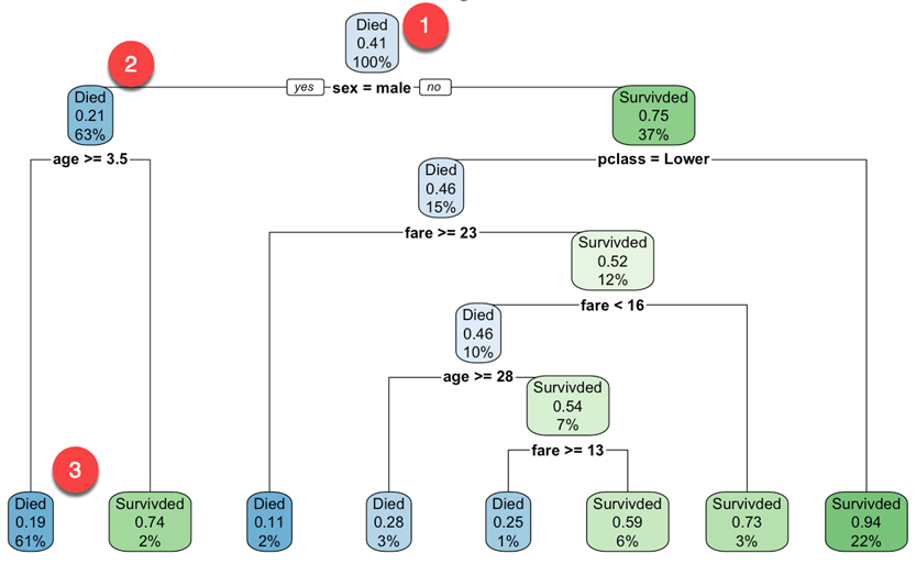
你从根节点开始(深度为 0/3,即图的顶部)。
- 顶部是整体的生存概率。它显示了在事故中幸存的乘客比例。41% 的乘客幸存下来。
- 该节点询问乘客的性别是否为男性。如果是,则向下移动到根节点的左子节点(深度 2)。63% 的乘客是男性,生存概率为 21%。
- 在第二个节点,你询问男性乘客的年龄是否大于 3.5 岁。如果是,则生存几率为 19%。
- 你可以继续这样理解哪些特征会影响生存的可能性。
请注意,决策树的优点之一是它们需要很少的数据准备。特别是,它们不需要特征缩放或居中。
默认情况下,rpart() 函数使用基尼不纯度度量来分割节点。基尼系数越高,节点内的实例差异越大。
步骤 5) 进行预测
你可以预测你的测试数据集。要进行预测,你可以使用 predict() 函数。R 决策树的 predict 基本语法是:
predict(fitted_model, df, type = 'class')
arguments:
- fitted_model: This is the object stored after model estimation.
- df: Data frame used to make the prediction
- type: Type of prediction
    - 'class': for classification
    - 'prob': to compute the probability of each class
    - 'vector': Predict the mean response at the node level
你想预测测试集中哪些乘客在碰撞后更有可能幸存下来。这意味着,你将知道在这 209 名乘客中,哪些人会生还或不会。
predict_unseen <-predict(fit, data_test, type = 'class')
代码解释
- predict(fit, data_test, type = ‘class’): 预测测试集的类别(0/1)。
测试未幸存的乘客和幸存的乘客。
table_mat <- table(data_test$survived, predict_unseen)
table_mat
代码解释
- table(data_test$survived, predict_unseen): 创建一个表格来计算与正确的 R 决策树分类相比,有多少乘客被分类为生还者和死亡者。
输出
##      predict_unseen
##        No Yes
##   No  106  15
##   Yes  30  58
模型正确预测了 106 名死亡乘客,但将 15 名生还者错误地归类为死亡。类比来说,模型错误地将 30 名乘客归类为生还者,而他们实际上是死亡的。
步骤 6) 评估性能
你可以使用混淆矩阵来计算分类任务的准确率度量。
混淆矩阵是评估分类性能的更好选择。基本思想是计算将真实实例分类为假的次数。
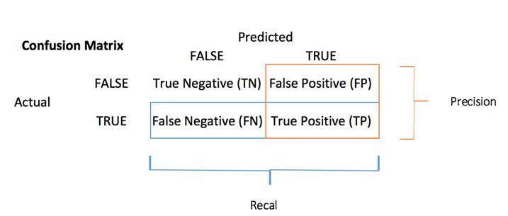
混淆矩阵中的每一行代表一个实际目标,而每一列代表一个预测目标。此矩阵的第一行考虑了死亡的乘客(False 类):106 人被正确分类为死亡(真阴性),而其余一人被错误地归类为生还者(假阳性)。第二行考虑了生还者,阳性类为 58 人(真阳性),而假阴性为 30 人。
你可以从混淆矩阵计算准确率测试。
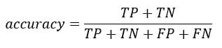
它是真阳性与真阴性之和除以矩阵总和的比例。在 R 中,你可以这样编码:
accuracy_Test <- sum(diag(table_mat)) / sum(table_mat)
代码解释
- sum(diag(table_mat)):对角线之和。
- sum(table_mat):矩阵之和。
你可以打印测试集的准确率。
print(paste('Accuracy for test', accuracy_Test))
输出
## [1] "Accuracy for test 0.784688995215311"
你的测试集得分为 78%。你可以对训练数据集重复相同的练习。
步骤 7) 调整超参数
R 中的决策树具有控制拟合各个方面的各种参数。在 rpart 决策树库中,你可以使用 rpart.control() 函数来控制参数。在以下代码中,你将介绍将要调整的参数。你可以参考 vignette 以了解其他参数。
rpart.control(minsplit = 20, minbucket = round(minsplit/3), maxdepth = 30)
Arguments:
-minsplit: Set the minimum number of observations in the node before the algorithm perform a split
-minbucket:  Set the minimum number of observations in the final note i.e. the leaf
-maxdepth: Set the maximum depth of any node of the final tree. The root node is treated a depth 0
我们将按以下步骤进行:
- 构建返回准确率的函数
- 调整最大深度
- 调整节点在分裂前必须具有的最小样本数
- 调整叶节点必须具有的最小样本数
你可以编写一个函数来显示准确率。你只需包装之前使用的代码即可。
- 预测:predict_unseen <- predict(fit, data_test, type = ‘class’)
- 生成表格:table_mat <- table(data_test$survived, predict_unseen)
- 计算准确率:accuracy_Test <- sum(diag(table_mat))/sum(table_mat)
accuracy_tune <- function(fit) {
    predict_unseen <- predict(fit, data_test, type = 'class')
    table_mat <- table(data_test$survived, predict_unseen)
    accuracy_Test <- sum(diag(table_mat)) / sum(table_mat)
    accuracy_Test
}
你可以尝试调整参数,看看是否能改进模型相对于默认值的性能。作为提醒,你需要获得高于 0.78 的准确率。
control <- rpart.control(minsplit = 4,
    minbucket = round(5 / 3),
    maxdepth = 3,
    cp = 0)
tune_fit <- rpart(survived~., data = data_train, method = 'class', control = control)
accuracy_tune(tune_fit)
输出
## [1] 0.7990431
使用以下参数:
minsplit = 4
minbucket= round(5/3)
maxdepth = 3cp=0
你获得了比之前模型更高的性能。恭喜!
摘要
我们可以总结在 R 中训练决策树算法的函数:
| 库 | 目标 | 函数 | 类 | 参数 | 详情 |
|---|---|---|---|---|---|
| rpart | 训练 R 中的分类树 | rpart() | class | formula, df, method | |
| rpart | 训练回归树 | rpart() | anova | formula, df, method | |
| rpart | 绘制树 | rpart.plot() | 拟合模型 | ||
| base | predict | predict() | class | fitted model, type | |
| base | predict | predict() | prob | fitted model, type | |
| base | predict | predict() | vector | fitted model, type | |
| rpart | 控制参数 | rpart.control() | minsplit | 设置算法执行分割前节点中必须存在的最小观测值数量。 | |
| minbucket | 设置最终节点(即叶节点)中必须存在的最小观测值数量。 | ||||
| maxdepth | 设置最终树任何节点的 maximum depth。根节点被视为深度 0。 | ||||
| rpart | 使用控制参数训练模型 | rpart() | formula, df, method, control |
注意:在训练数据上训练模型,并在未见过的数据集(即测试集)上测试性能。